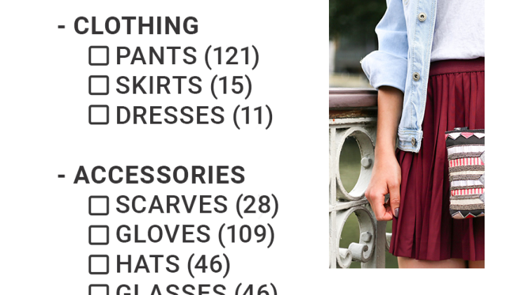
Faceting is the mechanism behind the filter boxes shown alongside search results in web shops and catalogs: each box lists a value that can narrow the result set and the number of items that value would leave. Implementing it in an application splits into two conceptual steps. First, reduce a universe of things to the current result — the base query. Second, pull out of that matched set the attributes and values usable for further narrowing, the facets themselves.
Facet types
Given a document-style schema, a typical distribution to expose covers type, category, start and end timestamps, size and tags.
|
1 2 3 4 5 6 7 8 9 10 |
CREATE TABLE documents ( id int4 primary key, created timestamptz not null, finished timestamptz, category_id int4 not null, tags text[], type mimetype, size int8, title text ); |
type is the simplest case: every distinct value becomes a facet, counted as type=application/pdf (1234). category_id behaves much the same at the counting level, except the category name has to be looked up for display. Hierarchical categories are a visualization concern rather than a counting one.
Categorical, continuous, composite
type and category_id are categorical variables: they take a limited, relatively small set of values, and can be counted as facets with no transformation. The remaining attributes belong to another class.
Continuous variables are those where nearly every row carries a unique value, with some values close together and others far apart. A unique facet per row is useless, so the standard treatment is bucketing: divide the value space into chunks and treat each chunk as a categorical value. Timestamps collapse into a month or year, size collapses into arbitrary ranges such as small, medium and large.
tags form a composite variable, since one result row contributes more than one facet value. Their counts do not sum to the number of result rows, and — the inverse consideration — selecting one tag does not exclude the others.
Counting facets with plain SQL
The naive approach runs the search query, then groups by the facet value and counts:
|
1 2 3 4 5 |
SELECT type, COUNT(*) FROM documents WHERE ... GROUP BY 1; SELECT category_id, COUNT(*) FROM documents WHERE ... GROUP BY 1; SELECT date_trunc('month', started), COUNT(*) FROM documents WHERE ... GROUP BY 1; SELECT date_trunc('month', finished), COUNT(*) FROM documents WHERE ... GROUP BY 1; SELECT width_bucket(size, array[0,1000,5000,10000,50000,100000,500000]), COUNT(*) FROM documents WHERE ... GROUP BY 1; |
tags needs a variant that unwraps the values; storing tags in an association table instead would follow a more traditional model without changing much:
|
1 |
SELECT tag, COUNT(*) FROM documents, LATERAL unnest(tags) tag WHERE ... GROUP BY 1; |
Three drawbacks follow. The query must be re-executed once per faceted attribute. There is heavy repetition between those queries. And generic handling of the results on the client side is difficult. PostgreSQL offers no way to return multiple result sets from a single query.
Collecting all facets in one result set
Getting every facet in one result set requires a concession: because the SQL type system has no variable data types, everything must be cast to text. Accepting that, a lateral subquery can emit the facets present in each matched row:
|
1 2 3 4 5 6 7 8 9 10 11 12 |
SELECT facet_name, facet_value, COUNT(*) FROM documents, LATERAL (VALUES ('type', type::text), ('category_id', category_id::text), ('created', date_trunc('month', created)::text), ('finished', date_trunc('month', finished)::text), ('size', width_bucket(size, array[0,1000,5000,10000,50000,100000,500000])::text) UNION ALL SELECT ) facets(facet_name, facet_value) WHERE ... GROUP BY 1, 2; |
The base query runs as before, and for each row the lateral part produces intermediary rows shaped as facet_name, facet_value. Grouping on that pair and counting gives the facet counts.
This performs reasonably at small result set sizes. Dynamically generating the query lets you skip facets already filtered down to a single value. At tens to hundreds of thousands of rows, though, response times become noticeable, and at roughly half a million matching results execution goes above 1 second even with many parallel workers. Over hundreds of millions of documents, matching a large fraction of them can push execution into minutes.
Inverted indexes as the fast path
The technique behind quick facet counts at scale is to store data so that intersecting the row lists matching a condition and sizing the result is cheap. That is what inverted indexes do: for each facet value they hold a list of matching documents. This approach is implemented in a PostgreSQL extension called pgfaceting, which uses roaring bitmaps through a PostgreSQL wrapper extension. Facets whose index should be precalculated have to be declared up front:
|
1 2 3 4 5 6 7 8 9 10 11 12 |
CREATE EXTENSION pgfaceting; SELECT faceting.add_faceting_to_table( 'documents', key => 'id', facets => array[ faceting.datetrunc_facet('created', 'month'), faceting.datetrunc_facet('finished', 'month'), faceting.plain_facet('category_id'), faceting.plain_facet('type'), faceting.bucket_facet('size', buckets => array[0,1000,5000,10000,50000,100000,500000]) ] ); |
Underneath, the extension builds a user space inverted index table listing matching documents per facet value. Composite facets are not yet supported but are planned. Index size stays modest: on a 100M document demo dataset, the inverted index comes out at 1% of the table size.
Because the index stands on its own, it can also resolve the base query result set quickly — selecting 60M rows and counting the results takes 155ms, without parallelism, on a single core.
|
1 2 3 4 5 6 7 8 9 10 11 12 13 |
SELECT facet_name, count(distinct facet_value), sum(cardinality) FROM faceting.count_results('documents'::regclass, filters => array[row('category_id', 24)]::faceting.facet_filter[]) GROUP BY 1; facet_name | count | sum ------------+-------+---------- created | 154 | 60812252 finished | 154 | 60812252 size | 7 | 60812252 type | 8 | 60812252 (4 rows) Time: 155.228 ms |
Further material is planned on reproducing this performance, handling hierarchical data, parallel index builds and incremental maintenance. The pgfaceting extension has just been released, and its query API is a stand-in for a considered implementation; early releases should be expected to change the API, require rebuilds between upgrades and carry other rough edges. Feedback on the desired shape of the API is welcome, as is hands-on contribution.