

Bringing PostGIS Data into QGIS
After loading OpenStreetMap data into PostGIS, the next step is visualization. QGIS connects directly to PostgreSQL/PostGIS without extra plugins, so you can pull in OSM layers quickly. To follow along you'll need a PostGIS-enabled database preloaded with OSM data (via osm2pgsql), a running QGIS client, and a Git client if you want to fetch pre-made style definitions.
Start by defining a new PostgreSQL connection in QGIS, open the database catalog, and add the layers you need. QGIS reads the geometry_columns view to determine the geometry type, spatial reference identifier, and dimensionality for each layer. Querying that view shows what the client sees:
|
1 2 3 |
select f_table_name as tblname, f_geometry_column as geocol, coord_dimension as geodim, srid, type from geometry_columns where f_table_schema = 'osmtile_iceland'; |
| tblname | geocol | geodim | srid | type |
| planet_osm_point | way | 2 | 3857 | POINT |
| planet_osm_line | way | 2 | 3857 | LINESTRING |
| planet_osm_polygon | way | 2 | 3857 | GEOMETRY |
| planet_osm_roads | way | 2 | 3857 | LINESTRING |
For geometry-typed columns, QGIS further checks geometrytype to confirm the actual geometry type modifier:
select distinct geometrytype(way) from planet_osm_polygon;
Default Styling to Start With
QGIS applies basic styling based on geometry type as soon as layers are added. The result is a raw, unstructured overview of points, lines, and polygons, which is only a starting point. Because the OSM import used a default style with no transformations, the data sits in three main tables — planet_osm_point, planet_osm_line, and planet_osm_polygon — without semantic filtering. It's up to the map designer to decide which features matter at a given zoom level and build rules that extract them.
A practical workflow for turning raw OSM data into readable cartography:
- Understand OSM's tagging model
- Decide which feature categories matter and at what scales
- Write queries that select only relevant records
- Convert those queries into QGIS rule expressions
- Iterate on visual quality and rendering performance
Take amenities as an example. Filtering for representative types shows how varied tags are stored across the layer:
|
1 |
select amenity, count(amenity) as amenityCount from planet_osm_point group by amenity order by amenityCount desc; |
| amenity | count |
| waste_basket | 1346 |
| bench | 1285 |
| parking | 479 |
| … |
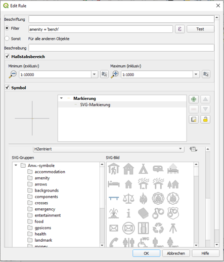
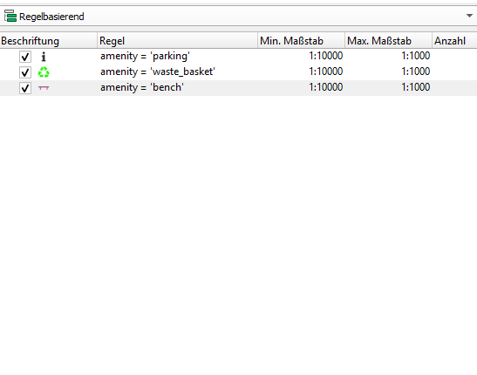
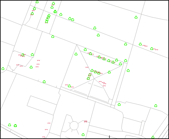
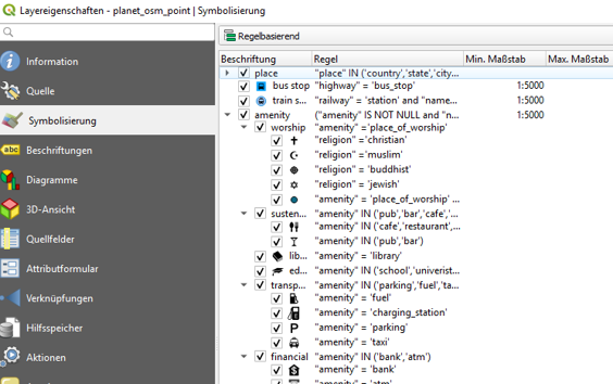
To style those points individually, open the layer properties, switch to rule-based symbology, then add a rule per amenity type. Each rule needs a query expression, a visible scale range, and a symbol (e.g., an SVG marker). The map updates based on the current viewport, so zooming reveals the styled features only at appropriate levels.
| Step 1 | Step 2 | Step 3 |
 |  |  |
Performance Checks on the Backend
Rendering delays often originate server-side. To see what QGIS actually sends to PostgreSQL, enable logging in postgres.conf and inspect the recorded statements. Running EXPLAIN ANALYZE on those queries exposes missing indexes.
|
1 2 3 4 5 6 |
EXPLAIN analyse SELECT st_asbinary("way", 'NDR'), ctid, "amenity"::text FROM "osmtile_iceland"."planet_osm_point" WHERE ("way" && st_makeenvelope(-2393586.56126631051301956, 9304920.7589644268155098, -2320619.86041467078030109, 9356509.49658409506082535, 3857)) AND (((("amenity" = 'parking') OR ("amenity" = 'waste_basket')) OR ("amenity" = 'wrench'))) |
In a typical case, the plan shows that planet_osm_point_way_idx (the spatial index on the way column) is used for bounding-box lookups, but no index exists on the amenity column — which slows down tag-based filters. Adding one helps:
|
1 2 3 4 5 6 7 8 9 10 11 |
Bitmap Heap Scan on planet_osm_point (cost=136.95..2272.97 rows=47 width=47) (actual time=0.537..1.239 rows=10 loops=1) Recheck Cond: (way && '0103000020110F000001000000050000001093D747F94242C1C46F49186BBF61411093D747F94242C15404E4AF9BD86141641122EE75B441C15404E4AF9BD86141641122EE75B441C1C46F49186BBF61411093D747F94242C1C46F49186BBF6141'::geometry) Filter: ((amenity = 'parking'::text) OR (amenity = 'waste_basket'::text) OR (amenity = 'wrench'::text)) Rows Removed by Filter: 4096 Heap Blocks: exact=74 Buffers: shared hit=115 -> Bitmap Index Scan on planet_osm_point_way_idx (cost=0.00..136.94 rows=3821 width=0) (actual time=0.495..0.495 rows=4106 loops=1) Index Cond: (way && '0103000020110F000001000000050000001093D747F94242C1C46F49186BBF61411093D747F94242C15404E4AF9BD86141641122EE75B441C15404E4AF9BD86141641122EE75B441C1C46F49186BBF61411093D747F94242C1C46F49186BBF6141'::geometry) Buffers: shared hit=41 Planning Time: 0.301 ms Execution Time: 1.276 ms |
For ongoing diagnostics, the auto_explain extension logs expensive statements automatically, which is a faster alternative to manual log inspection.
Adopting Community Styles
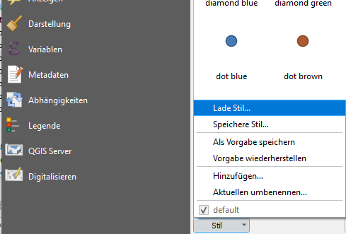
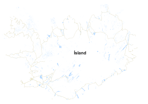
Building a full OSM style from scratch is heavy work. To speed up the process you can grab existing layer settings — for instance, the public Beautiful_OSM_in_QGIS repository — and load them per layer via the layer properties. That yields a familiar OSM-like rendering that you can then tweak for your own purpose.
| Step 1 | Step 2 |
 |  |
 | 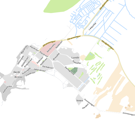 |
Keep in mind that visual complexity isn't free. Missing scale restrictions, costly expressions, and absent indexes all translate directly into slow map loading. The public OSM style is highly detailed and correspondingly expensive to render, so any customization should weigh readability against the resources it consumes.
Summary
Connecting PostGIS to QGIS is straightforward, and the default styling is enough for quick orientation. Real usability comes from targeted rule-based styles and attention to what the database has to support them — the right indexes, clean queries, and scale-sensitive rules keep maps responsive as you add detail.