
OpenSky-Network has been collecting air traffic surveillance data since 2013 and releases it free of charge for non-commercial use, which makes it a practical playground for spatio-temporal analysis. The walkthrough below takes a day of that data through PostgreSQL, PostGIS and MobilityDB, from import to trajectory construction to a handful of flight queries.
Toolchain
A current PostgreSQL installation with PostGIS and MobilityDB is the core requirement; older releases of both also work, and a prebuilt container image is available at https://registry.hub.docker.com/r/codewit/mobilitydb for those who would rather not build MobilityDB themselves. Raw flight data arrives as large csv files, so ogr2ogr from the gdal package handles the copy into the database. QGIS serves as the visualization client.
The setup used here: Ubuntu 20.04.3, PostgreSQL 13, PostGIS 3.2.1, MobilityDB 1.0.0, ogr2ogr 3.0.4 and QGIS 3.20.3.
Loading a day of state vectors
OpenSky publishes snapshots of the previous Monday's complete state vector data covering the last six months. Each state vector carries time (one-second update interval), icao24, lat/lon, velocity, heading, vertrate, callsign, onground, alert/spi, squawk, baro/geoaltitude, lastposupdate and lastcontact. The sample analysis uses the 24 csv files for 2022-02-28.
A fresh database with the PostGIS and MobilityDB extensions provides the store:
|
1 2 3 4 5 6 7 8 9 10 11 12 13 14 15 16 17 |
postgres=# create database flightanalysis; CREATE DATABASE postgres=# c flightanalysis You are now connected to database 'flightanalysis' as user 'postgres'. flightanalysis=# create extension MobilityDB cascade; NOTICE: installing required extension 'postgis' CREATE EXTENSION flightanalysis=# dx List of installed extensions Name | Version | Schema | Description ------------+---------+------------+------------------------------------------------------------ mobilitydb | 1.0.0 | public | MobilityDB Extension plpgsql | 1.0 | pg_catalog | PL/pgSQL procedural language postgis | 3.2.1 | public | PostGIS geometry and geography spatial types and functions (3 rows) |
The OpenSky dataset description supplies the structure for a staging table that holds unaltered raw vectors:
|
1 2 3 4 5 6 7 8 9 10 11 12 13 14 15 16 17 18 19 20 21 22 23 24 25 26 |
create table tvectors ( ogc_fid integer default nextval('flightsegments_ogc_fid_seq'::regclass) not null constraint flightsegments_pkey primary key, time integer, ftime timestamp with time zone, icao24 varchar, lat double precision, lon double precision, velocity double precision, heading double precision, vertrate double precision, callsign varchar, onground boolean, alert boolean, spi boolean, squawk integer, baroaltitude double precision, geoaltitude double precision, lastposupdate double precision, lastcontact double precision ); create index idx_points_icao24 on tvectors (icao24, callsign); |
Importing from a directory of uncompressed csv files runs like this:
for f in ls *.csv; do
ogr2ogr -f PostgreSQL PG:"user=postgres dbname=flightanalysis" $f -oo AUTODETECT_TYPE=YES -nln tvectors --config PG_USE_COPY YES
done
The staging table ends up with 52,261,548 rows.
Building trajectories
MobilityDB models movement through temporal types such as tgeompoint, a temporal geometry point. To use it, native position rows first become trajectories:
|
1 2 3 4 5 6 7 8 9 10 11 12 13 14 15 |
create table if not exists flightsegments ( icao24 varchar not null, callsign varchar not null, trip tgeompoint, traj geometry(Geometry,4326), constraint flightsegment_2_pkey primary key (icao24, callsign) ); create index idx_trip on flightsegments using gist (trip); create index idx_traj on flightsegments using gist (traj); |
Individual flights are tracked by selecting vectors by icao24 and callsign, ordered by time. Because the staging table stores time as a unix timestamp, converting to timestamps with time zone is a convenient first step:
|
1 2 3 4 5 |
update tvectors set ftime= to_timestamp(time) AT TIME ZONE 'UTC'; create index idx_points_ftime on tvectors (ftime); |
The trajectories themselves come from aggregating locations by icao24 and callsign in time order:
|
1 2 3 4 5 6 7 8 |
insert into flightsegments(icao24, callsign, trip) SELECT icao24, callsign, tgeompoint_seq(array_agg(tgeompoint_inst(ST_SetSRID(ST_MakePoint(Lon, Lat), 4326), ftime) ORDER BY ftime)) from tvectors where lon is not null and lat is not null group by icao24, callsign; |
QGIS has no native support for tgeompoint, so raw geometries must be extracted for display. Applying st_simplify to the trajectory yields a lighter geometry; MobilityDB's own simplification methods operate on the whole trajectory rather than only its geometry:
|
1 2 |
update flightsegments set traj = st_simplify(trajectory(trip)::geometry, 0.001)::geometry; |
A first look at the data
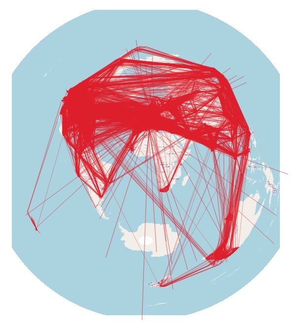
Even a single day of freely available vectors is a lot of data, and the visualization makes that plain. It also shows why cleansing matters: coverage and recording gaps produce trajectories that span the globe, and those in turn produce wrong and misleading results. That filtering step is left out here in favour of working within a small geographic area.
Querying the trajectories
With trajectories in place, several questions can be answered directly in SQL.
Distinct airframes
Counting distinct aircraft by icao24:
|
1 2 |
select count(distinct icao24) from flightsegments; |
|
1 2 3 4 5 |
flightanalysis=# select count(distinct icao24) from flightsegments; count ------- 41663 (1 row) |
Average flight duration
|
1 2 3 4 5 |
flightanalysis=# select avg(duration(trip)) from flightsegments where st_length(trajectory(trip::tgeogpoint)) > 0; avg ----------------- 03:50:48.245525 (1 row) |
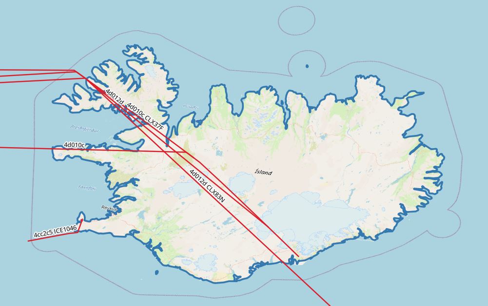
Vectors crossing Iceland between 2022-02-28 00:00:00+00 and 2022-02-28 03:00:00+00
This requires country borders, downloadable from Natural Earth and imported first.
|
1 2 3 4 5 6 7 8 9 10 |
select icao24, callsign, trajectory(atPeriod(T.Trip, '[2022-02-28 00:00:00+00, [2022-2-28 03:00:00+00]'::period)) FROM flightsegments T, ne_10m_admin_0_countries R WHERE T.Trip && stbox(R.geom, '[2022-02-28 00:00:00+00, [2022-02-28 03:00:00+00]'::period) AND st_intersects(trajectory(atPeriod(T.Trip, '[2022-02-28 00:00:00+00, [2022-2-28 03:00:00+00]'::period)), r.geom) and R.name = 'Iceland' and st_length(trajectory(atPeriod(T.Trip, '[2022-02-28 00:00:00+00, [2022-2-28 03:00:00+00]'::period))::geography) > 0 |
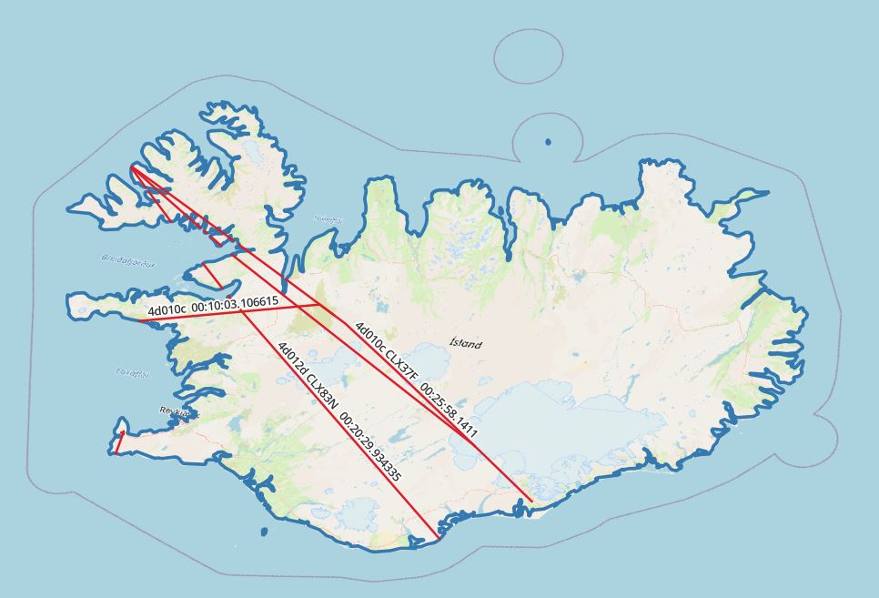
Flyover duration over the same window
|
1 2 3 4 5 6 7 8 9 10 11 12 13 14 15 16 17 18 19 |
select icao24, callsign, (duration( (atgeometry((atPeriod(T.Trip::tgeompoint, '[2022-02-28 00:00:00+00, [2022-02-28 03:00:00+00]'::period)), R.geom))))::varchar, trajectory( atgeometry((atPeriod(T.Trip::tgeompoint, '[2022-02-28 00:00:00+00, [2022-02-28 03:00:00+00]'::period)), R.geom)) FROM flightsegments T, ne_10m_admin_0_countries R WHERE T.Trip && stbox(R.geom, '[2022-02-28 00:00:00+00, [2022-02-28 03:00:00+00]'::period) AND st_intersects(trajectory(atPeriod(T.Trip, '[2022-02-28 00:00:00+00, [2022-2-28 03:00:00+00]'::period)), r.geom) and R.name = 'Iceland' and st_length(trajectory(atPeriod(T.Trip, '[2022-02-28 00:00:00+00, [2022-2-28 03:00:00+00]'::period))::geography) > 0 |
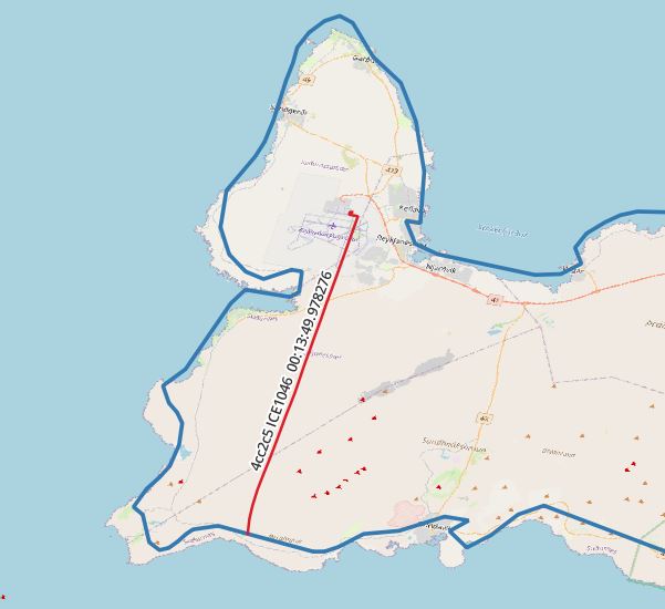
Border crossings for a given airframe and callsign
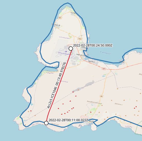
For the case shown, the aircraft did not leave the country during the trip.
|
1 2 3 4 5 6 7 8 9 10 11 12 13 14 15 16 17 18 19 20 21 22 23 24 25 26 27 |
with segments as ( select icao24, callsign, unnest(sequences( atgeometry( (atPeriod(T.Trip::tgeompoint, '[2022-02-28 00:00:00+00, [2022-02-28 03:00:00+00]'::period)), R.geom))) segment FROM flightsegments T, ne_10m_admin_0_countries R WHERE T.Trip && stbox(R.geom, '[2022-02-28 00:00:00+00, [2022-02-28 03:00:00+00]'::period) AND st_intersects(trajectory(atPeriod(T.Trip, '[2022-02-28 00:00:00+00, [2022-2-28 03:00:00+00]'::period)), r.geom) and R.name = 'Iceland' and trim(callsign) = 'ICE1046' and st_length(trajectory(atPeriod(T.Trip, '[2022-02-28 00:00:00+00, [2022-2-28 03:00:00+00]'::period))::geography) > 0) select icao24,callsign, st_startpoint(getvalues(segment)), st_endpoint(getvalues(segment)), starttimestamp(segment), endtimestamp(segment) from segments |
Where this leads
MobilityDB's feature set removes much of the manual effort from spatio-temporal analysis, and domains such as toll systems, surveillance and logistics are obvious candidates for it. The upcoming release is expected to open the door from research and testing to production use. The project has continued to develop since the earlier MobilityDB write-up, and a basic introduction to the extension is worth reading first for anyone new to it.