How to interpret PostgreSQL EXPLAIN ANALYZE output

Reading plans from a declarative engine

Because SQL is declarative, you state the result you want rather than the procedure that produces it. EXPLAIN exposes the execution plan produced by the optimizer, and EXPLAIN ANALYZE goes further: it runs the statement and reports the actual time and row count of every step. That combination is the starting point for statement-level tuning in PostgreSQL.

Note that a patch written for PostgreSQL 16, EXPLAIN GENERIC PLAN, has since been included in that release.

Choosing options

Options are passed in parentheses. The ones that matter most:

• ANALYZE executes the query and adds real timings and row counts per step. Because it executes, it is risky on UPDATE and DELETE.
• BUFFERS reports the 8kB blocks read, written and dirtied per step. It is valid only together with ANALYZE.
• VERBOSE prints the output expressions of each step. Usually clutter, but useful when time is burned inside a frequently called, expensive function.
• SETTINGS, available from v12, lists performance-relevant parameters that deviate from their defaults.
• WAL, introduced in v13, reports WAL usage for data-modifying statements and requires ANALYZE.
• FORMAT selects the output format. TEXT is the default and the most readable; XML, JSON and YAML suit automated processing.

The usual invocation is:

Add SETTINGS on v12 or later, and WAL for data-modifying statements from v13 on. Turning on track_io_timing is worthwhile because it yields I/O timing data.

Statement types and measurement caveats

EXPLAIN covers SELECT, INSERT, UPDATE, DELETE, EXECUTE of a prepared statement, CREATE TABLE ... AS and DECLARE of a cursor. Nothing else.

Instrumentation is not free: EXPLAIN ANALYZE adds measurable overhead, so a slower runtime is expected. Execution times also vary between runs, particularly on a first execution when the data is not yet cached, which makes repeated runs worth the effort.

What the output contains

Without options

Plain EXPLAIN shows the estimated cost, the estimated row count and the estimated width of an average result row. Cost is expressed in an artificial unit where reading an 8kB page during a sequential scan counts as 1. Each node carries two values: startup cost to produce the first row and total cost to produce them all.

With ANALYZE

A second parenthesis adds actual execution time in milliseconds, actual row count, and the loop count — how many times the node ran — along with the number of rows eliminated by filters.

The footer reports planning and execution time for the whole statement, and SUMMARY OFF suppresses it.

With BUFFERS

Per node you get the blocks found in cache (hit), those read from disk, those written and those dirtied. Recent versions extend the footer with the same figures for optimizer work when it could not satisfy its reads from cache. With track_io_timing = on, I/O operations also carry timing data.

Cost, time and loops in a tree

A plan is a tree of nodes. The top node appears first; deeper nodes are indented and prefixed with ->. Equal indentation means equal level, as with the two relations joined together.

Execution proceeds top down. The executor asks lower nodes for rows on demand, pulling only what the upper node needs to compute its next row. Consequently, the startup time of an upper node is never below that of its children, and the same applies to total time. Net time for a node therefore requires subtracting the time consumed by its children, a calculation that parallel queries complicate further. Both cost and time must also be multiplied by the loop count to get the total spent in a node.

Where to look first

Three signals carry most of the diagnostic value:

• The nodes consuming the largest share of execution time.
• The lowest node where estimated and actual row counts diverge sharply — a factor of roughly 10 is the usual threshold. A bad estimate at one node frequently explains a slow plan elsewhere, because the plan choice was made on faulty numbers.
• Long sequential scans whose filter discards most of the rows, which are candidates for an index.

Visualizers

Long plans are hard to read as raw text, and two web tools render them graphically.

Depesz' visualizer

Available at https://explain.depesz.com/, it accepts a pasted plan and returns a layout close to the original but easier on the eye.

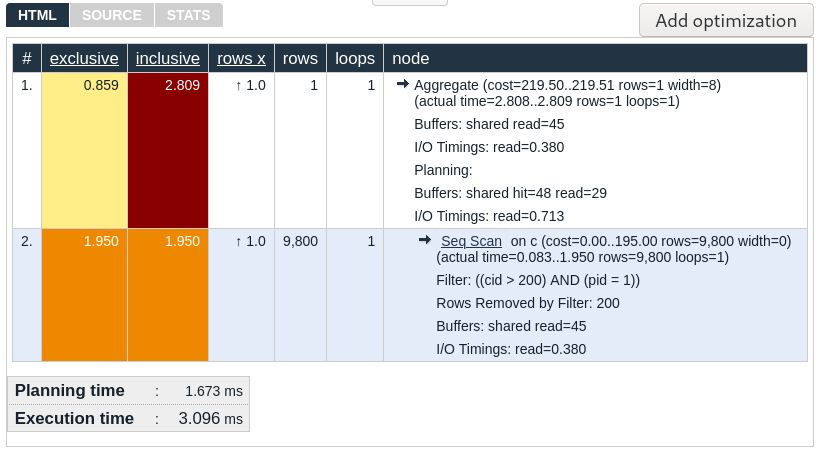
• Total and net execution time are computed per node, with the most expensive nodes highlighted in red.
• A “rows x” column gives the factor by which the row count was over- or underestimated, again with bad cases marked red.
• Clicking a node hides its subtree, which lets you skip irrelevant parts of a long plan.
• Hovering a node marks its direct children with a star so they can be located quickly.

The original EXPLAIN text stays visible once you have narrowed your attention to one node. The presentation is old-school, but the site has existed for a long time.

Dalibo's visualizer

At https://explain.dalibo.com/, a pasted plan is submitted in the same way and rendered as a tree.

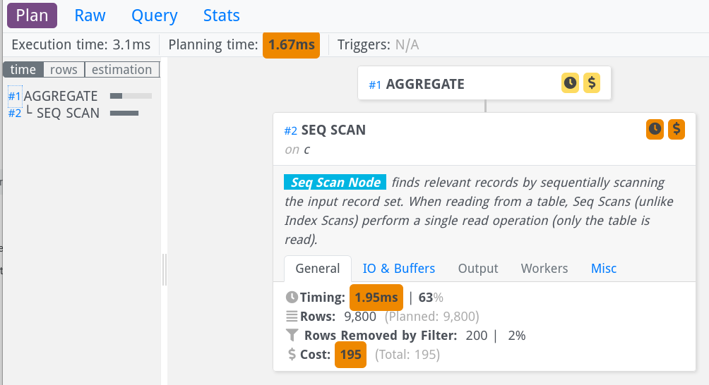
Details are collapsed initially and unfold on click, as with the second node shown above. A panel on the left lists all nodes and links to the detail view on the right.

• Bars on the left indicate relative net execution time, making the most expensive nodes stand out.
• Selecting “estimation” on the left shows the per-node row count error.
• Selecting “buffers” shows which nodes consumed the most 8kB blocks — informative, since those nodes' performance depends on how well the data is cached.
• On the right, a node expands into tabs with full detail.
• A crosshair icon in the lower right corner of a node collapses its subtree.

Its strength is making the plan's tree structure visually explicit, with a more current interface. The trade-off is that detail is hidden and has to be located.

In practice

EXPLAIN (ANALYZE, BUFFERS) with track_io_timing enabled delivers what is needed to diagnose statement performance, and Depesz' or Dalibo's visualizer keeps the resulting text manageable; their feature sets are broadly comparable. For parameterized statements, EXPLAIN(ANALYZE) deserves a closer look, and finding the statements worth tuning at all is a job for pg_stat_statements.