From Photo to Rectangular Scan
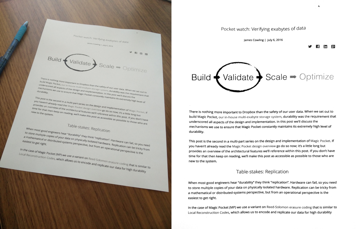
Dropbox’s document scanner lets users photograph a document on a phone and produce a clean, rectangular PDF, even when the original photo is rotated, slightly crumpled, or partly in shadow. The previous post covered how the system detects the document’s boundaries. Here we look at the two steps that follow: rectifying the detected quadrilateral into a rectangle, and enhancing the result for uniform illumination and crisp contrast.
On a flatbed scanner these effects come for free because the capture environment is tightly controlled. With a handheld camera, the document and camera can move freely, so the geometry must be estimated and the lighting must be corrected explicitly.
Undoing the Perspective Transform
The input document is physically rectangular, but when it is not facing the camera squarely, the detected corners form a general convex quadrilateral. To produce a rectangular output, we need to invert the geometric transform introduced by the capture process. That transform depends on the camera’s extrinsic parameters (position and orientation relative to the document), its intrinsic parameters (such as focal length), and the document’s physical dimensions.
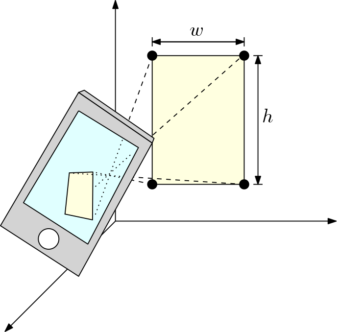
Assuming a symmetric camera (no skew or astigmatism), the unknowns are:
- the 3D camera position relative to the document (3 degrees of freedom),
- the 3D camera orientation (3 degrees of freedom),
- the document dimensions (2 degrees of freedom), and
- the camera focal length (1 degree of freedom).
The x- and y-coordinates of the four detected corners provide eight constraints. Although this leaves nine unknowns, the system is not underdetermined: a physical scaling of the document plus a corresponding change in camera distance yields the identical photo, effectively adding a constraint. The result is a fully determined system, and once the parameters are recovered, the perspective transform can be inverted.
Mapping each output pixel back to the source image can be slow, but GPUs are designed for exactly this kind of texture rendering. The view transform that renders the rectified document is the inverse of the camera transform we just solved for. In practice, the ambiguity of scale remains: we cannot tell whether the document is letter paper or a poster board. The system resolves this by counting the pixels inside the detected quadrilateral and matching the output resolution to that count, avoiding excessive upsampling or downsampling.
Enhancement as an Optimization Problem
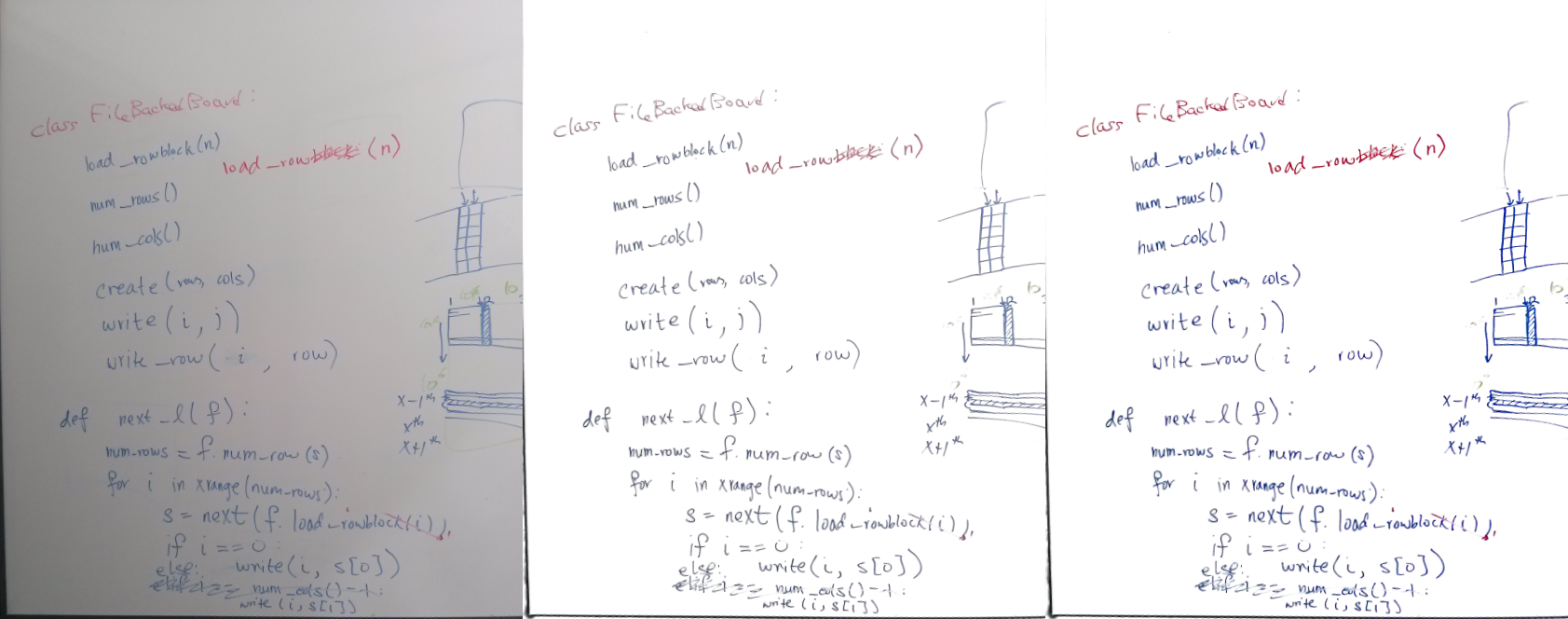
With a rectangular rendering in hand, the goal is a clean, evenly lit scan. We can treat enhancement explicitly as an optimization problem: solve for an output image J(x,y) derived from the input I(x,y) that best meets two requirements — a mostly uniform white background, and foreground text and figures that are sharp and high-contrast.
If we could label every pixel as foreground or background, the task would be simple, but binary labels introduce aliasing on small text. A single global linear transform also fails because shadows and uneven lighting vary across the image. Instead, the system writes a cost function that penalizes undesirable output, then runs a standard optimization.
The cost for the first requirement (a white background) is straightforward: compare the output to a constant white value (255), and minimize the deviation across all pixels:

For the second requirement, we need to preserve local structure while removing global brightness changes. A common measure of local structure is the image gradient — the difference between neighboring pixels. The cost is then the degree to which the output gradient differs from the original:

Combining the two costs yields a system equivalent to Poisson’s equation, which is well known in computer graphics and physics. It can be solved efficiently via conjugate gradient descent or the fast Fourier transform. The implementation relies on Apple’s Accelerate framework and open-source templating libraries such as Eigen and Dropbox’s own Lopper.
Speeding Up the Solver
Solving Poisson’s equation at full resolution (8–12 megapixels on recent iPhones) can still take seconds on older devices, and a multi-page PDF multiplies the wait. To make the user experience smoother, the goal is to cut processing time by an order of magnitude.
A useful observation is that, locally, the output is nearly a linear function of the input. If we apply a local gain and offset, we get a good solution in small regions:

But there is no single gain and offset that works for the entire image—that is why the Poisson machinery was needed in the first place. To accommodate shadows and uneven illumination, we let the gain and offset vary across the image:

This formulation is more flexible, but it doubles the unknowns: now we must solve for gain and offset at every pixel rather than a single output value. The key constraint is that the gain and offset should vary slowly across the image; we are correcting lighting, not patterned paper. This lets us solve at a much lower resolution than the input — vastly faster — and then upsample the gain and offset fields back to the original resolution. The low-resolution solution also implicitly enforces local correlation. Once the gain and offset are known everywhere, they are combined with the input to produce the final output image.
Preserving Color
All the derivations above ignore color, but the input is usually RGB. Applying the algorithm independently to each channel can create color shifts because the channels are no longer constrained together. An initial approach substituted original RGB values back into pixels that were not close to white, but this produced colors that looked faded. The reason is visual color constancy: the human visual system judges brightness relatively, so colors that look vivid against dark input look washed out against a bright white background.
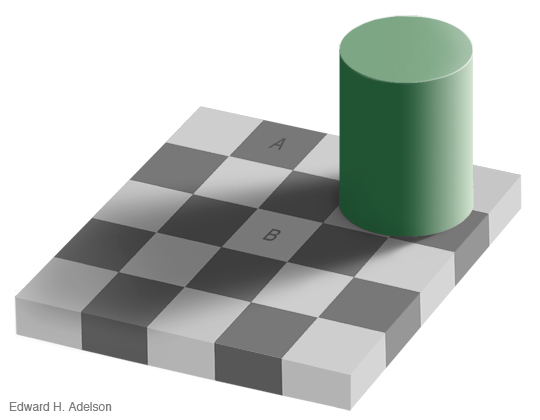
To prevent this effect, the algorithm converts the image to HSV color space and copies the hue and saturation from the original where appropriate. The gains and offsets are applied only to the value channel, which yields a much better color appearance.
Dealing with Imperfect Detections
The rectification step assumes the document detection returned a perfect quadrilateral. In practice, many documents have edges that are not perfectly straight, and corners may be dog-eared. The rectified image can therefore include background regions that are not part of the document. These are detected and removed using a simple graph min-cut algorithm, which segments out well-delineated dark areas near the borders, yielding an output that better matches what the user intended.
A Tunable Result
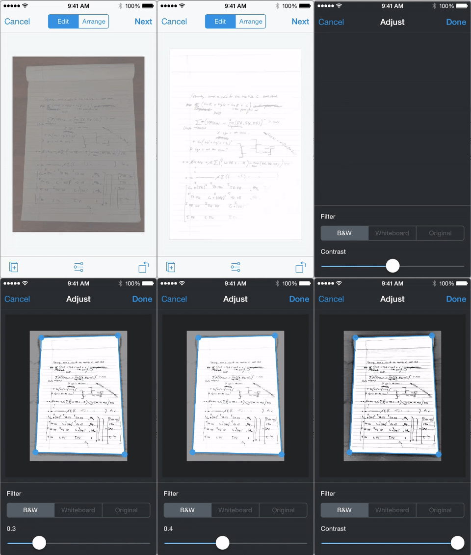
The full pipeline starts with a detected document boundary, rectifies it, and then enhances for readability. The enhancement algorithm includes a single user-facing contrast parameter (along with the relative weighting of the cost terms, such as k1 and k2), which is exposed through a simple interface. This lets users dial in exactly the appearance they want from the scanner.
Making the pipeline fast enough for real-time use
With the rectification and enhancement approach settled, the next challenge was purely practical: making it run quickly enough to feel instant inside the Dropbox mobile app. The target was under 200 ms on a modern phone, which ruled out any multi-stage architectures that would require multiple full-resolution passes. The solution hinged on a three-part strategy: shrinking the input for the most expensive work, moving the final warping step into native code, and tuning the backend to process four output pixels at a time.
Downscaling the heavy lifting
The first optimization was simple but effective: run the document segmentation network on a much smaller version of the image. Instead of feeding the model the full-resolution photo, the input is downscaled to a width of 320 pixels before inference. The segmentation maps produced by the model — the boundary and foreground probability maps — are still full-size in spirit, but they are cheap to compute at this lower resolution and then upscaled. Because the network only needs enough detail to locate the document and classify the regions, small and blurry does not hurt the result.
Detecting the page boundary next becomes a far smaller problem. The corner-to-corner and boundary refinement both run on a low-resolution percentile analysis rather than the full image. Corner priors are extracted globally using the percentile-based heuristics, while local boundary refinement is done in a narrow band around a first coarse estimate. Every step works at reduced scale, which keeps the total cost down to a fraction of what the original frame would require.
Rendering with OpenGL instead of the NPU
The most time-consuming part in early benchmarks was actually the warping and blending itself. For that stage the team offloaded the work to OpenGL rather than trying to run it through the mobile neural processing unit. The GPU is an ideal fit for the image transformation, since each output pixel's value is an independent computation — there are no cross-pixel dependencies to serialize.
The whole rendering pass happens in native code with a single fragment shader. Each shader invocation covers two-by-two pixel blocks, matching the four-channel RGBA output of the color enhancement network. This makes the pipeline fully parallel: one thread per four-pixel group, with no dependency between groups. The OpenGL path performs the bilinear sampling of the input, the look-up table (LUT) based color correction, the lighting model for surface slant, the local sharpening, and the background floor map application — all in one pass per intermediate stage. Blending the document with the cleaned background is a separate, equally light pass.
The white point for surface-shading correction is estimated on the small downscaled image as well, using the RGB values around the detected page border rather than the page text. Those border pixels are averaged to get a reliable baseline, which prevents the correction from being skewed by bright characters inside the document.
Sharing intermediate arrays between the segmentation engine on the neural processing unit and the OpenGL shader adds a small element of overhead, but the result of all these decisions is a pipeline that consistently finishes in around 150-250 ms on the phones the team tested.
The architecture also makes the memory footprint fairly small. All of the images are fixed-size buffers, and every stage reads from one or two sources and writes to one destination. If the phone does not support OpenGL ES 3.0, the app reads back the warped buffer at reduced resolution and falls back to a simpler CPU-based rendering path with the same steps.
Testing and integration
Validation of the system relied on an internal photo benchmark that tests the pipeline's performance and accuracy on a set of representative document photos. New builds were run against this benchmark table, allowing the team to compare frame time, precision, and a reconstruction metric across versions. The reconstruction metric measured how well the automatically enhanced and rectified document resembled a flat, evenly lit original — with lower average error indicating better quality.
For clean inputs, the enhancement stage often dominates the pipeline. For more difficult shots, the segmentation and corner resolution step costs as much as the enhancement. This is fine in practice, because the whole pipeline stays within the latency budget.
The feature ships today in the Dropbox mobile apps on both iOS and Android, and it is one of two document scanner article offerings the team discusses separately. The other, which uses a larger compute budget, is covered in another report.