Why Facebook’s web tier needs dynamic sizing
The web tier that serves Facebook.com traffic is a global service spread across many data centers. User activity follows time-of-day patterns, so global load rises and falls with the number of active people. Peak demand generally coincides with evening hours in Europe and Asia while much of the Americas is still awake; the trough comes later in the evening on the U.S. West Coast. Because the global load balancer, Taiji, keeps regional load levels similar, every data center follows the same peak-and-valley curve.
Static provisioning required the web tier to hold enough capacity year-round to cover peak demand, an extra disaster recovery (DR) buffer for losing the largest data center region, projected engagement growth, and other operational headroom. That meant many machines sat idle during off-peak hours. The previous manual process also required larger safety margins because adding capacity took time.
With autoscaling, the web tier is sized dynamically each day. Capacity is removed outside peak hours and restored before demand rises, while individual machines continue running at load levels comparable to peak-time utilization. The gap between peak and off-peak demand is large, so the freed machines become available for other purposes, including machine learning workloads. The shift has been in production for two years; its safety depends on accurate throughput modeling, which is the core reason this approach is preferred over other sizing techniques.
Throughput versus utilization metrics
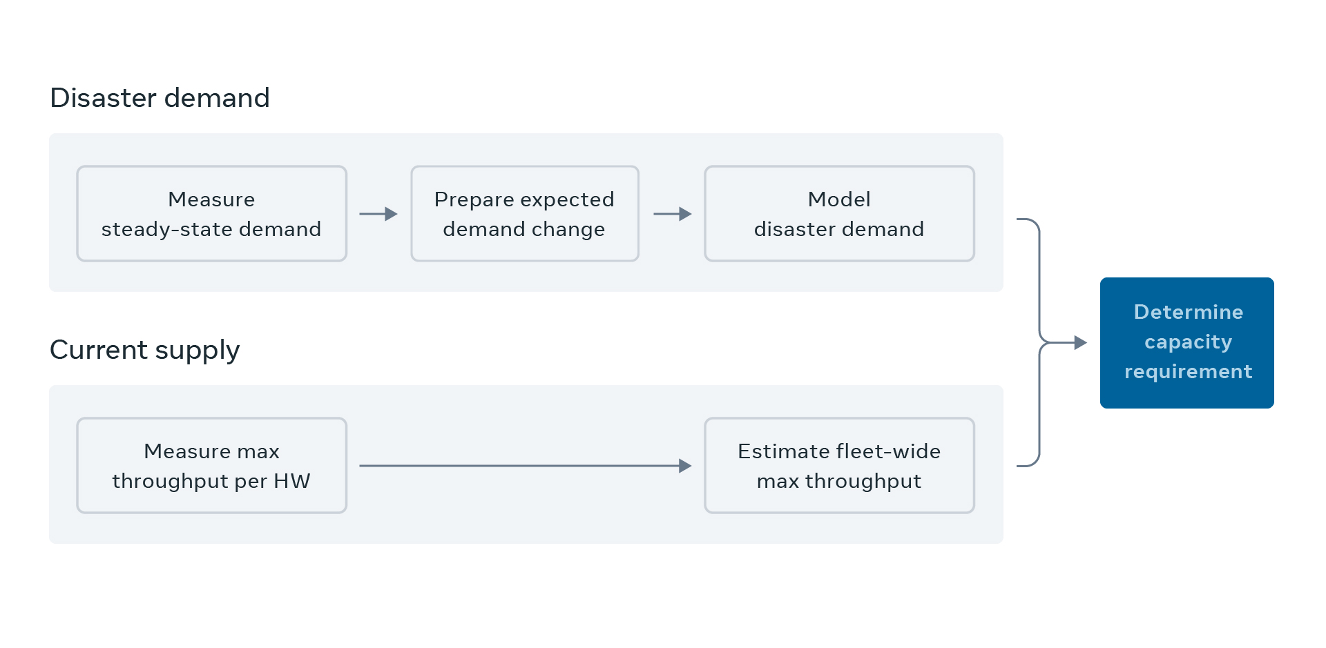
Throughput autoscaling makes sizing decisions based on the absolute amount of work a service performs. Requests per second (RPS) is a common throughput metric, though for ML services that rank elements, the number of elements ranked per second better captures the actual useful work. Throughput differs from utilization, which is a normalized measure of system load and therefore changes with server count. Throughput is independent of server count, which makes it suitable for estimating two quantities:
- Current supply: total throughput a service can handle with its current capacity in a given region.
- Disaster demand: throughput required when a region must absorb demand from a lost data center region.
The autoscaler compares supply and disaster demand and adjusts the number of hosts so that capacity meets demand without a large surplus. A key advantage is that this method models required capacity for workloads that have not yet been seen historically — something utilization-based approaches cannot do.
Predicting steady-state and disaster demand
Estimation of disaster demand begins with measured steady-state demand. Throughput metrics such as QPS are gathered per server and aggregated to regional totals. Historical measurements train ML models to recognize seasonal patterns, which are then queried during capacity modeling to predict future demand. Model outputs are cross-checked against live measurements to catch deviations from historical behavior.
Predicted demand improves safety by increasing capacity ahead of time when future growth is expected, and it helps services with long startup or shutdown times. Predictions also stabilize autoscaling by suppressing high-frequency fluctuations; for example, a binary push on the web tier causes elevated warmup traffic, and rapid capacity changes between pushes would be unnecessary.
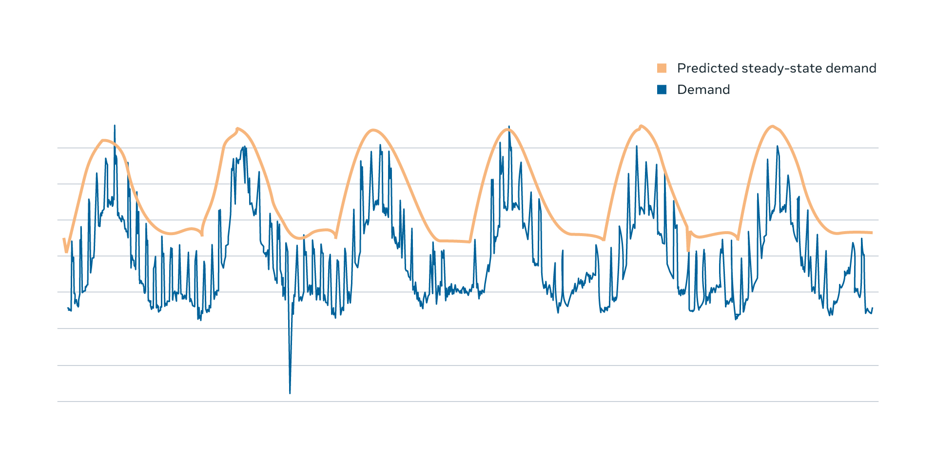
Predicted demand is then adjusted for expected changes, such as client feature launches, holidays, or infrastructure maintenance that alters regional traffic.
Disaster readiness adds another layer. Disasters — from networking outages to weather events — can degrade an entire data center region with little notice. When that happens, Taiji redistributes the region’s traffic to the remaining regions in proportion to each region’s size. To estimate disaster demand, autoscaling simulates the loss of the largest data center region and computes the extra demand each surviving region would receive. This incremental demand is summed with predicted steady-state demand to produce the disaster demand value used for sizing.
Measuring supply with load tests
Demand estimates are only useful if actual hosting capacity is known. Each current deployment has a maximum throughput before performance degrades — for example, error rates or latency become unacceptable. That maximum is the throughput supply. Sizing adjusts the container count so that supply stays as close to disaster demand as possible without falling below it.
Supply is measured with an internal load testing platform that gradually moves organic production traffic to a small set of target hosts. Real traffic gives a more accurate picture than simulated load. The tests monitor target hosts and back off once a degraded state appears; data from just below the degradation threshold establish each host’s maximum safe throughput.
These load tests run continuously throughout the day, covering each region and hardware profile a service uses. Per-machine measurements are aggregated into a regional supply estimate at a given moment. If supply is too low or too high relative to predicted disaster demand, the load test data guide how many machines to add or remove.
How the pieces combine
A simplified example shows the workflow for a service deployed in three regions — U.S. West, U.S. East, and Europe:
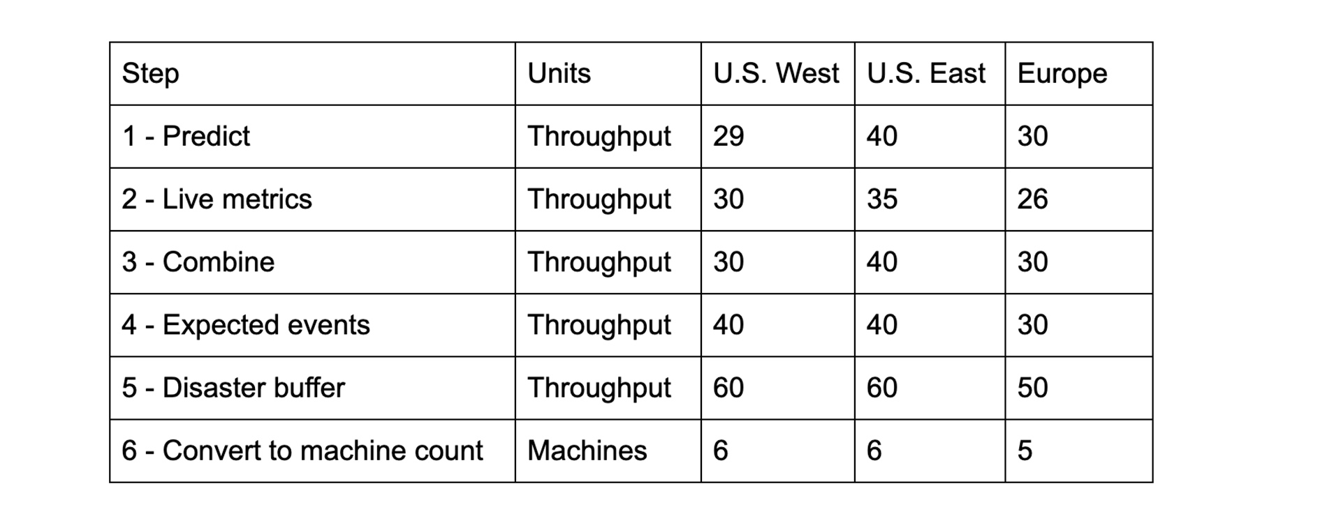
- Query ML models for predicted demand in the next hour.
- Query live state. In this example every region is below prediction except U.S. West.
- Aggregate predictions with measurements, choosing the maximum of the two for safety. That means predictions are used in most regions; live metrics are used only in U.S. West.
- Account for imminent infrastructure changes. Suppose a traffic shift moves 25 percent of U.S. East demand to U.S. West. Since the shift has not happened yet, current U.S. East demand must still be covered, so only the U.S. West prediction is adjusted upward.
- Apply the disaster buffer. Assuming each region redistributes equally to the other two, the loss of U.S. West would add 20 demand units to both U.S. East and Europe; similarly, U.S. East’s loss adds 20 units to U.S. West. Each region therefore must hold a 20-unit disaster buffer.
- Convert demand to machine count. If load tests show 10 demand units per machine, the final per-region size is computed by simple division.
The example intentionally omits load balancer behavior, hardware profile differences, and other regional effects that matter in production but would obscure the core sizing logic.
Validating the capacity model
A capacity model is only useful if its errors are understood and bounded. That starts with the throughput metric itself, which must measure useful work uniformly. Queries per second (QPS) fails this test for most services: in the web tier, serving the News Feed requires far more work than resolving a deep link to a single post. When request costs are not uniform across infrastructure, a shift toward cheaper requests makes capacity look ample while a shift toward expensive requests silently overloads the service.
Metric quality issues propagate through every stage of the model—measured supply, historical and current demand, and future predictions. Supply measurements carry load-testing error, demand estimates carry ML prediction error, and simulations of load balancer behavior add their own uncertainty. Rather than trust an end result that might hide offsetting mistakes, the system validates individual steps. For example, steady-state demand predictions are compared against actual demand during normal periods. Because predictions are meant to be conservative, the focus is on intervals where actual demand exceeded the prediction.
End-to-end validation happens through specific scenarios. Disaster drills, which disconnect an entire data center region from the production network, provide a realistic setting to compare pre-disaster capacity estimates against observed behavior. Hardware turn-ups and decommissions offer similar comparison points.
Building the autoscaling ecosystem
The capacity model answers one question: what size should the service be? Turning that answer into a safe, reliable resizing operation requires an entire system around it. The controller must change container counts without compromising service health, detect its own failures as human oversight decreases, and return freed capacity to other workloads.
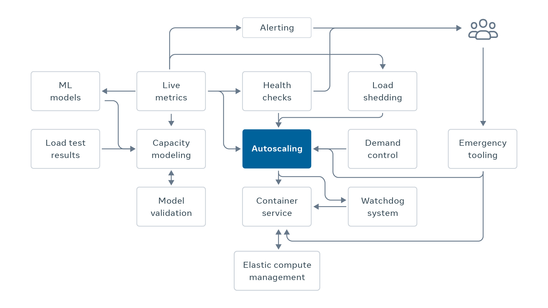
Safety mechanisms
Dynamic sizing is efficient—the web tier's diurnal pattern makes that clear—but it adds a new dependency on automation working quickly and correctly. Several failure modes are possible:
- Demand exceeds the disaster prediction due to an unexpected surge or a prediction error.
- The autoscaling automation goes down and cannot upsize before peak.
- The autoscaling automation misbehaves and downsizes too aggressively off-peak.
The system layers multiple defenses against these risks.
Reactive fallback
Predictive autoscaling, based on the disaster demand forecast, always runs alongside a reactive algorithm. The reactive path measures current throughput demand, adds a small buffer percentage, and computes a desirable size from that. Throughput autoscaling takes the larger of the two sizes. In normal operation the predictive size wins because it can upsize ahead of an expected demand increase. The reactive size only dominates when current demand spikes far beyond recent daily patterns, serving as a failsafe when demand approaches supply.
Watchdog
An auxiliary watchdog service monitors the heartbeat from autoscaling. If no heartbeat arrives within a configured interval, the watchdog restores capacity to a safe size—typically the maximum of the last seven days. This is a last line of defense against catastrophic failure, so it is deliberately simple and dependency-free. It also shares no code with autoscaling itself, since a bad binary release in the main automation is a likely cause of failure.
Sizing verification and small steps
Autoscaling depends on input data quality—load testing results, hardware mix, and other sources. A verification stage checks this data and assigns a confidence level to each capacity estimate. Unstable load test measurements or insufficient data points lower the confidence, which halts autoscaling and triggers the watchdog to return capacity to the safe level.
During resizing, additional checks validate each step: resize completion within a desired time window, service health during downscales, cross-region traffic status (to avoid shrinking a service that is shedding load), and overall service size (to prevent downsizing into a deficit). Any anomaly reverts the service to its original size.
Downscaling also proceeds in small, configurable steps—for example, a maximum change of 5 percent of total service capacity per 15-minute window. Small steps give health checks and alerting time to detect an undersized service before it becomes critical.
Dynamic sizing in production
With these mechanisms in place, the Facebook web tier has run under dynamic sizing for over a year. The savings are substantial: the web tier is large and its peak-to-trough difference is significant, so off-peak hours free a considerable number of servers. These servers flow into the elastic compute pool, which holds machines not currently needed by their original workloads. Its size varies as machines enter and leave.
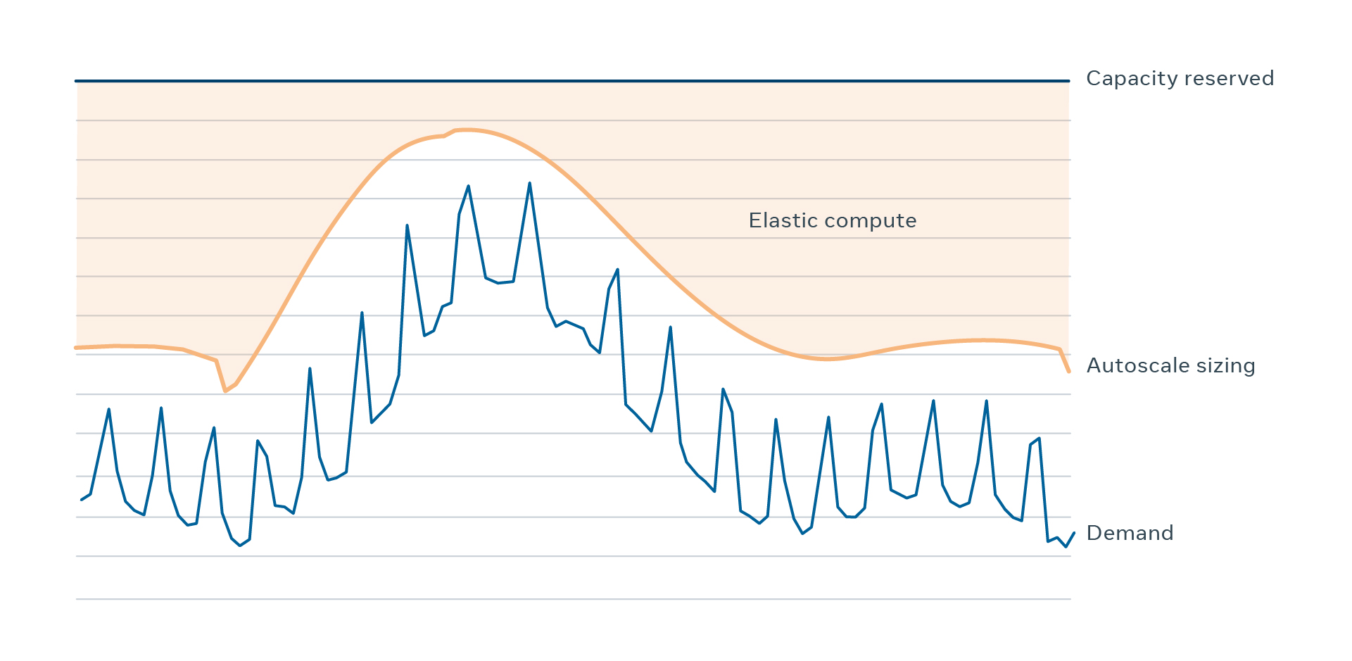
Elastic compute pool users are typically short-lived, latency-insensitive jobs that run asynchronously: time-shifted async jobs, ML model training, feed ranking improvements, ad optimization, and harmful content detection. These workloads previously required dedicated capacity; now they fill servers that would otherwise sit idle during web off-peak hours.
Scaling beyond the web tier
Following the web tier's year-long success, the same methodology is now being applied to other large services with diurnal patterns—the Django web service for Instagram and multifeed services, among others. As autoscaling adoption grows, more servers enter the elastic compute pool, opening opportunities for workloads to migrate from permanently dedicated capacity to elastic allocation.
The combination of autoscale and elastic compute lets infrastructure run closer to actual demand. That efficiency supports the increasing compute needs of new products across Facebook, Instagram, and WhatsApp—including the critical ML workloads that now take advantage of previously unused capacity.