Why Routing Is Hard
Building a routing system that spans multiple machines means accepting that failures are not exceptional—they’re structural. Nodes crash, networks partition, and the system rarely fails all at once. More often, you get partial degradation: two nodes unable to reach each other while a client can see both, nodes lying about their state, or clock skew that makes time appear to move backward.
The CAP theorem frames the tradeoff: of consistency, availability, and partition tolerance, you can guarantee two. Partitions are common enough in real infrastructure that refusing to operate during one is effectively an availability failure. So you pick CP or AP—or some probabilistic middle ground—and live with the consequences.
Safety and liveness offer a complementary lens. Liveness means there’s always a path to the “right thing” happening—no deadlock, no infinite loop. Safety means the system never does anything bad. For HTTP request routing, the requirements look like this:
- The system must tolerate partitions.
- It must be as available as possible. A slow response beats no response.
- Requests can’t take forever—there’s a liveness bound.
- Requests must complete correctly or not at all. No double-POSTs, no dropped payloads. That’s the safety constraint.
There’s no perfect solution here. Nuclear loss of data centers ends availability regardless of design. Networks can lie in ways that make correctness impractical. The liveness bound is the only real lever: you can let latency climb to absorb failures, within reason.
And then there’s the human factor. Engineers have limited time, limited ability to reason about distributed state, and legacy systems that were never meant for this. At scale, complex algorithms are hard to prove and harder to predict. A dumb, predictable algorithm often beats an optimal but intricate one.
Injecting Faults Into the Simulation
To see how a routing stack behaves under stress, dynos in the simulation can be made to fail with the faulty function. A component stays online for an exponentially distributed time, then crashes and returns errors. After a second exponentially distributed outage, it recovers. This is a fail-fast model—the node returns failure immediately instead of hanging on to messages. For short-lived simulations, using relatively brief failure windows makes the dynamics visible.
(defn faulty-dyno []
  (cable 2
    ; Mean time before failure of 20 seconds, and
    ; mean time before resolution of one second.
    (faulty 20000 1000
      (queue-exclusive
        (delay-fixed 20
          (delay-exponential 100
            (server :rails))))))
With a pool of 250 dynos under Poisson-distributed load, comparing an even load balancer against a pool of perfect dynos versus faulty ones is revealing:
(test-node "Reliable min-conn -> pool of faulty dynos."
  (lb-min-conn
    (pool pool-size
      (faulty-dyno)))))
.                     Ideal dynos       95% available dynos
Total reqs:           100000            100000
Selected reqs:        50000             50000
Successful frac:      1.0               0.62632
Request rate:         678.2972 reqs/s   679.6156 reqs/s
Response rate:        673.90894 reqs/s  676.74567 reqs/s
Latency distribution:
Min:                  24.0              4.0
Median:               93.0              46.5
95th %:               323.0             272.0
99th %:               488.0             438.0
Max:                  1044.0            914.0
The result is counterintuitive: a pool that’s 95% available still fails more than a third of all requests. The reason is the load balancer itself. Faulty nodes fail immediately, which leaves their queues shorter on average, and the min-conns balancer responds by routing more traffic to them.
Real load balancers like HAProxy track failures and avoid them. Instead of active health checks, a simpler passive scheme works in simulation: when a request fails, don’t decrement that host’s connection counter right away. Wait about one second—the mean time to resolution for a dyno. The error response still returns immediately, preserving fail-fast behavior, but the balancer becomes less likely to assign new requests to a broken node.
(lb-min-conn :lb {:error-hold-time 1000}
  (pool pool-size
    (faulty-dyno)))))
Total reqs:       100000
Selected reqs:    50000
Successful frac:  0.98846
Request rate:     678.72076 reqs/s
Response rate:    671.3302 reqs/s
Latency distribution:
Min:     4.0
Median:  92.0
95th %:  323.0
99th %:  486.0
Max:     1157.0
Throughput dips slightly from the perfect-pool baseline, but reliability climbs to 98% from a pool of nodes that is only 95% available, with no meaningful latency penalty. The system is now more reliable than its constituent parts.
There’s an inherent bound here: some requests must fail so the system can learn which dynos are up. Retrying at the load balancer level—up to three total requests—pushes availability higher still:
(test-node "Retry -> min-conn -> faulty pool"
  (retry 3
    (lb-min-conn :lb {:error-hold-time 1000}
      (pool pool-size
        (faulty-dyno))))))
Total reqs:       100000
Selected reqs:    50000
Successful frac:  0.99996
Request rate:     676.8098 reqs/s
Response rate:    670.16046 reqs/s
Latency distribution:
Min:     12.0
Median:  94.0
95th %:  320.0
99th %:  484.0
Max:     944.0
Combining retries, least-conns balancing, and steering clear of failing nodes yields 99.996% availability with negligible latency impact. That’s a solid building block—but it doesn’t yet scale.
Scaling Out the Routers
Min-conns and round-robin balancers depend on coordinated state. If the balancer itself lives on faulty hardware, one option is to distribute it for high availability. But that requires low-latency state coordination, which the CAP theorem rules out. The alternative is probabilistic tradeoffs under partitions, like permitting duplicate requests to reach the same backend.
Another approach: punt on AP min-conns entirely. Make each balancer a single machine or a CP cluster that fails completely when it hits a problem.
(defn faulty-lb
  [pool]
  (faulty 20000 1000
    (retry 3
      (lb-min-conn :lb {:error-hold-time 1000}
        pool))))
Back to a Bamboo-like model: a stateless random routing layer on top sends requests to 10 faulty least-conns balancers, all routing over one shared pool of faulty dynos:
(test-node "Random -> 10 faulty lbs -> One pool"
  (let [dynos (dynos pool-size)]
    (lb-random
      (pool 10
        (cable 5
          (faulty-lb
            dynos)))))))
Total reqs:       100000
Selected reqs:    50000
Successful frac:  0.9473
Request rate:     671.94366 reqs/s
Response rate:    657.87744 reqs/s
Latency distribution:
Min:     10.0
Median:  947.0
95th %:  1620.0
99th %:  1916.0
Max:     3056.0
Availability drops to 95% in this two-layer design. The cause is state isolation. The least-conns routers share nothing, so they can’t tell each other which dynos are down. Requests get sent to broken backends more often. A balancer that actively checked state would avoid this, but a second retry layer above the random routing works too:
(let [dynos (pool pool-size (faulty-dyno))]
      (retry 3
        (lb-random
          (pool 10
            (cable 5
              (faulty-lb
                dynos))))))))
Total reqs:       100000
Selected reqs:    50000
Successful frac:  0.99952
Request rate:     686.97363 reqs/s
Response rate:    668.2616 reqs/s
Latency distribution:
Min:     30.0
Median:  982.0
95th %:  1639.0
99th %:  1952.010000000002
Max:     2878.0
Latency doesn’t improve, but availability reaches three nines—respectable for a stateless layer over a 95% available pool.
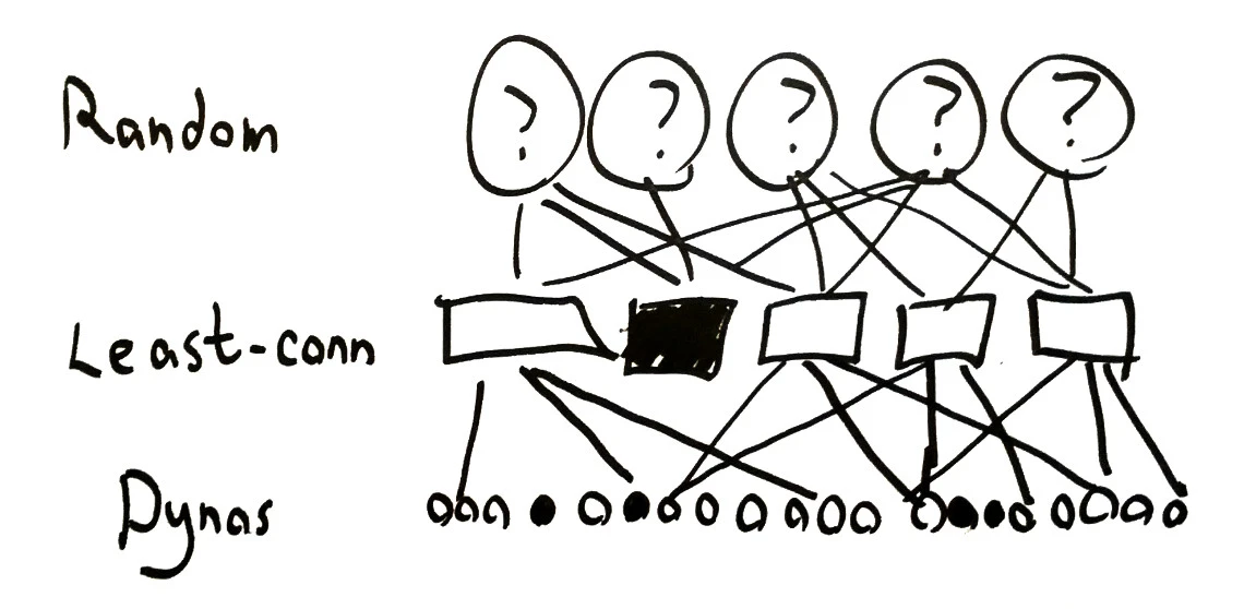
Isolating the least-conns routers preserves liveness. The cost: they can’t coordinate efficient allocation, so they encounter extra failures and queue messages on the same dynos independently. One fix is giving each least-conns router a complete view of its backends by isolating the dyno pools:
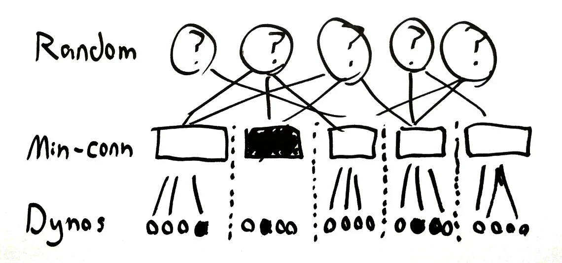
There are real tradeoffs. Random routing can load one block’s router more than its peers, and those routers can’t forward to dynos outside their block. Worse, since these routers are CP systems, a router failure takes out its whole dyno block. Design becomes a balance: more dynos per block improves least-conns efficiency; more blocks limits the blast radius of a router outage.
With 10 blocks of 25 dynos each:
  (test-node "Retry -> Random -> 10 faulty lbs -> 10 pools"
    (retry 3
      (lb-random
        (pool 10
          (cable 5
            (faulty-lb
              (pool (/ pool-size 10)
                (faulty-dyno)))))))))
Total reqs:       100000
Selected reqs:    50000
Successful frac:  0.99952
Request rate:     681.8213 reqs/s
Response rate:    677.8099 reqs/s
Latency distribution:
Min:     30.0
Median:  104.0
95th %:  335.0
99th %:  491.0
Max:     1043.0
Availability still sits at 99.9% with a stateless random layer atop 10 routers that are each 95% available. Throughput drops a bit, but median latency improves ninefold over the homogeneous pool.
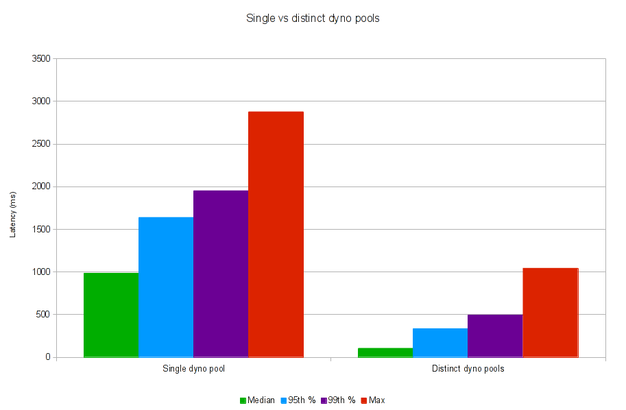
The lesson in distributed design is composition. Each component—whether an efficient but unscalable CP system or a scalable but inefficient AP one—is complex on its own. Enforce simple guarantees per component, then combine them into larger systems. This architecture pairs an efficient (but nonscalable) CP balance layer with an inefficient (but scalable) AP routing layer, and gets a useful hybrid.
This only works if the topology cooperates. Dynos should sit close to their least-conns balancer—ideally one per rack, connected to the rack’s switch—so correlated failures stay within the smallest possible network area. On EC2, without clear network boundaries, correlated failures across blocks are a genuine risk. And the design assumes single-threaded, queuing backends. Concurrent servers—a growing share of Heroku’s hosted apps—don’t fit this model well. Dynamic pools, where dynos spin up and down constantly, remain an open problem as well.