Reverse mode Automatic Differentiation - Eli Bendersky's website

Reverse-Mode Automatic Differentiation Explained

Automatic Differentiation (AD) computes exact derivatives for arbitrary programs by systematically applying the chain rule along a computational graph. Two flavors exist: forward mode, which propagates derivatives from inputs outward, and reverse mode, which works backward from outputs. Reverse mode is the generalization of backpropagation used for neural network training and works for graphs with multiple outputs, not just scalar loss functions.

The essential prerequisite is fluency with the multivariate chain rule, since real computations rarely form simple linear pipelines.

Starting Simple: Linear Graphs

A clean test case is the sigmoid function, which is a single-input, single-output composition.

In Python, we can build this up from primitives:

def sigmoid(x):
    f = -x
    g = math.exp(f)
    w = 1 + g
    v = 1 / w
    return v

This computation can also be drawn as a graph where each box is a primitive operation and edges carry values between them:

We want the derivative of the final value S with respect to input x evaluated at a specific point . Running the graph forward with x = gives:

Because every operation has exactly one input and one output, the single-variable chain rule suffices. Reverse mode peels the composition from the output backward. The last step, from S to v, has derivative 1 since S = v exactly. Then the next layers give:

• dS/dv = 1
• dv/dw = e^−w/(1+e^−w)², evaluated at w from the forward pass
• Continue backward through the remaining primitives until the input is reached

At x = 0, this yields dS/dx = 0.24 — matching the analytic derivative. The process is purely mechanical, which makes it easy to automate. But real graphs are rarely linear, so the general case of directed acyclic graphs (DAGs) needs multivariate algebra.

General Graphs, General Chain Rule

A function with n inputs mapping to m outputs has a Jacobian matrix of partial derivatives:

When composing functions, the multivariate chain rule multiplies their Jacobians:

This is a plain matrix product between the Jacobian of the outer function and the Jacobian of the inner function . The concrete cases of interest for reverse mode are nodes with a single input (linear), multiple inputs (fan-in), and outputs that feed multiple consumers (fan-out).

Linear Nodes

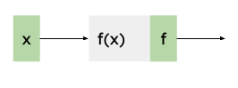
For a node with one input and one output, the Jacobian is just its derivative, so the chain rule recovers the familiar single-variable form:

Fan-in: Multiple Inputs

When node f takes two inputs:

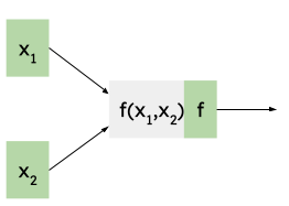
Its Jacobian is a 1×2 matrix. If the downstream derivative dS/df is already known as a scalar, the chain rule multiplies that 1×1 "matrix" against the row: https://cdn.eli.thegreenplace.net/images/math/7dd8f88c95647185fbf3b60fe0fe5d3f954cbf84.png

In plain terms, the derivative simply weights each input by its own partial derivative:

• dS/dx₁ = dS/df · ∂f/∂x₁
• dS/dx₂ = dS/df · ∂f/∂x₂

Fan-out: Shared Outputs

When the output of node f feeds two downstream consumers—even though the forward values are identical—the reverse derivative must treat them separately. The node thus behaves like a two-output function:

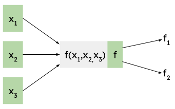
Its Jacobian for the two output edges is 2×n. Downstream derivatives arrive as a row of two values, and applying the chain rule gives: https://cdn.eli.thegreenplace.net/images/math/4af79fd8777d1e4a0990a887cb40fd27b1d9cced.png

This yields the crucial insight: contributions from each output edge add, so the sensitivity of any input is the sum of sensitivities computed along each separate output path.

Working a Complete DAG Example

Using a sample function from the ADIMLAS paper, the decomposition into primitives forms an interconnected graph:

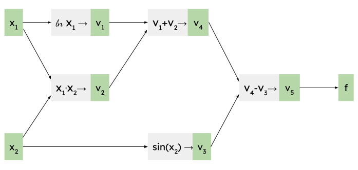
With inputs (a, b) = 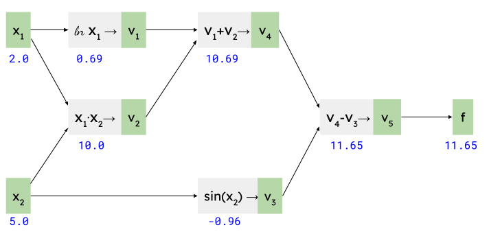, the forward pass computes all intermediate values. The reverse pass then flows from the output backward.

Starting from dS/dS = 1, each node applies the fan-in formulas. For nodes with multiple dependent children, we accumulate contributions incrementally as we move backward. A node like a sits at a fan-out position, so its final gradient is the sum of contributions from each downstream path it feeds:

Verifying with the analytical derivatives of the original expression confirms both gradients.

Why Backpropagation Prefers VJPs

Reverse mode is the natural choice for machine learning problems because they train toward a scalar loss—meaning we run AD exactly once per training example. Forward mode would instead need one full pass per input weight, which is impractical for models with millions of parameters.

The efficiency goes deeper: applying reverse mode amounts to computing a vector-Jacobian product (VJP). The chain rule for a node becomes:

But because the overall graph has a scalar output, the gradient arriving at any node is a row vector, not a full matrix. The product is again a row vector. AD libraries therefore never store complete Jacobians—each registered primitive supplies a VJP function instead. This matters because Jacobians are often huge and sparse; keeping them whole would be wasteful.

There is also a second way to think about efficiency. Working backward from the single output means intermediate results stay small—rows, not matrices. Working forward would multiply full Jacobians together at every step, generating large intermediate matrices before collapsing to the final gradient. Reverse mode sidesteps that blow-up entirely.

How a Minimal Reverse Mode AD Implementation Works

Reverse mode AD is straightforward to implement in code. A minimal Python implementation demonstrates the core ideas: building a computational graph as expressions are evaluated, then walking that graph backwards to compute gradients.

The API is simple: users construct expressions out of Var objects, then call grad() on the output node:

xx = Var(0.5)
sigmoid = 1 / (1 + exp(-xx))
print(f"xx = {xx.v:.2}, sigmoid = {sigmoid.v:.2}")

sigmoid.grad(1.0)
print(f"dsigmoid/dxx = {xx.gv:.2}")

Building the sigmoid expression and calling grad(1.0) on the output Var populates the gv attribute of the input Var with the correct derivative (0.24, matching hand calculation). The same pattern works for multi-node graphs:

x1 = Var(2.0)
x2 = Var(5.0)
f = log(x1) + x1 * x2 - sin(x2)
print(f"x1 = {x1.v:.2}, x2 = {x2.v:.2}, f = {f.v:.2}")

f.grad(1.0)
print(f"df/dx1 = {x1.gv:.2}, df/dx2 = {x2.gv:.2}")

Here, grad on the final node correctly propagates gradients backward to the input Vars involved in intermediate calculations.

Anatomy of a Var

A Var holds two pieces of state:

• v: the forward-computed value of the node.
• predecessors: a list of nodes feeding into it.

Each predecessor is a small structure containing a reference to the upstream Var and a multiplier representing the partial derivative of this node's output with respect to that predecessor's value.

@dataclass
class Predecessor:
    multiplier: float
    var: "Var"

Take the DAG example's node v5 = v4 - v3. Its predecessor list has two entries: one for v4 with multiplier 1 (since the derivative of v4 - v3 with respect to v4 is 1), and one for v3 with multiplier -1 (since the derivative with respect to v3 is -1). Operators and custom math functions construct these entries using derivatives of their respective operations.

def __add__(self, other):
    other = ensure_var(other)
    out = Var(self.v + other.v)
    out.predecessors.append(Predecessor(1.0, self))
    out.predecessors.append(Predecessor(1.0, other))
    return out

# ...

def __mul__(self, other):
    other = ensure_var(other)
    out = Var(self.v * other.v)
    out.predecessors.append(Predecessor(other.v, self))
    out.predecessors.append(Predecessor(self.v, other))
    return out

def log(x):
    """log(x) - natural logarithm of x"""
    x = ensure_var(x)
    out = Var(math.log(x.v))
    out.predecessors.append(Predecessor(1.0 / x.v, x))
    return out

def sin(x):
    """sin(x)"""
    x = ensure_var(x)
    out = Var(math.sin(x.v))
    out.predecessors.append(Predecessor(math.cos(x.v), x))
    return out

Notably, some derivative calculations require the forward values of input Vars at runtime. For example, the derivative of sin(x) is cos(x), so the Var implementation must store its input's value (x.v) to compute the multiplier when the graph is built.

The grad traversal

With the graph in place, grad performs a backward walk:

def grad(self, gv):
    self.gv += gv
    for p in self.predecessors:
        p.var.grad(p.multiplier * gv)

The method relies on several key details:

• Invocation target. grad must be called on the output Var representing the entire computation (the loss).
• Edge direction. The graph stores predecessors, not successors, so walking backward means starting from the output and moving toward the inputs via the predecessors list.
• Initial gradient. Typical use begins with grad(1.0) because the output node's own gradient with respect to itself is 1.
• Accumulation via self.gv += gv. This is essential for fan-out nodes: per the multivariate chain rule, if a node feeds into multiple downstream operations, the gradients from all output paths must be summed at that node.

This implementation is deliberately simplistic. In graph topologies where a node can be reached via multiple paths, the same Var may be visited multiple times during the traversal. Production systems sort the graph topologically first, visiting each node exactly once. A related limitation is that grad accumulates into gv, so a Var should not be reused across separate gradient computations.

Industrial AD frameworks such as autograd and JAX offer better performance and ergonomics, but they operate on the same principle: reverse mode differentiation over an explicit computational graph. The full toy implementation is available online.