Fourier analysis of infinite discrete signals relies on the Discrete-Time Fourier Series and Transform, but practical digital signal processing deals with signals that are both discrete and finite in duration. That constraint motivates the Discrete Fourier Transform.
From finite samples to frequency coefficients
Given a finite block of signal samples, the goal is the same as in the infinite case: find coefficients of a complex exponential series that reconstructs the signal. One approach treats the samples as a finite window into an otherwise zero-valued infinite signal and computes its DTFT. The problem is that the DTFT is a continuous function of frequency, so it cannot be evaluated and stored for every value on a real computer; some choice of frequencies to compute must be made.
A second approach avoids that choice entirely. The available samples can be treated as a single period of a periodic signal and analyzed with the DTFS, which reconstructs a discrete periodic signal exactly. Because the finite signal is just one period, a DTFS reconstructs it exactly as well. This equivalence is the core idea behind the DFT.
Definition and naming
By convention the transform is written with a normalization such that the forward coefficients come directly from the series coefficients. The word transform is used in its general mathematical sense of a mapping from one object to another: here, from the sample sequence to the sequence of coefficients.
Relation to the DTFT
The DFT and DTFT are tightly connected. The continuous-frequency obstacle of the DTFT is resolved by sampling that frequency variable in the discrete domain: the DFT amounts to N equally spaced samples of the DTFT.
Computing the transform
The correspondence between code and the summation formula is direct:
def dft(x):
    """Return X[k] = sum_n x[n] exp(-2 pi i k n / N)."""
    N = len(x)
    n = np.arange(N)
    X = np.empty(N, dtype=complex)
    for k in range(N):
        weights = np.exp(-2j * np.pi * k * n / N)
        X[k] = np.sum(x * weights)
    return X
NumPy's vectorization does the work — the weights array is computed in full for each k, because n is an array of indices.
The DFT matrix and roots of unity
Powers of the complex roots of unity form an orthogonal basis, which gives a linear algebra view of the transform. All N-th roots of unity are powers of a single one, and the conjugates of the roots are themselves roots, appearing in reversed order across the full enumeration.
Collecting the vectors formed by raising that root to integer powers from 0 to N−1 into a matrix yields a square matrix whose rows form an orthogonal basis. Multiplying a signal, viewed as a column vector, by this matrix produces exactly the DFT vector — each coefficient comes from a row–column product. The matrix is called the Fourier Matrix or DFT Matrix, and the same computation can be implemented as a matrix multiplication:
def dft_matrix(N):
    """Construct F[k, n] = W_N**(k*n), where W_N = exp(-2 pi i / N)."""
    # W_N is a primitive N-th root of unity: W_N**N = 1.
    # Its powers give all N roots of z**N - 1 = 0.
    root = np.exp(-2j * np.pi / N)
    indices = np.arange(N)
    # Rows correspond to frequency bins k; columns to sample indices n.
    exponents = np.outer(indices, indices)
    return root**exponents

def dft_via_matrix(x):
    """Compute the DFT as F @ x with the Fourier matrix"""
    return dft_matrix(len(x)) @ x
The construction mirrors the continuous case, where trigonometric functions — equivalently, complex exponentials — form an orthogonal basis for square-integrable functions. Here the basis lives in discrete space and can represent any sequence of N complex values.
Reconstructing the signal
The inverse DFT restores the original samples from the coefficients, and it can be derived two ways.
- From the DTFS reconstruction formula. Substituting the convention used for the forward transform directly yields the Inverse Discrete Fourier Transform expression.
- From the Fourier matrix. Every element of the conjugate matrix is the conjugate of the corresponding element of the Fourier matrix. Multiplying the Fourier matrix by this conjugate matrix gives the identity matrix, since the conjugate is the inverse; left-multiplying the DFT vector by it recovers the original signal. Written in summation form, this matches the DTFS-derived formula.
Both routes agree, and the linear algebra picture is clean: the roots-of-unity basis is orthogonal and the transform is invertible, so reconstructing a vector is just left-multiplication of its DFT by the conjugate matrix.
Worked example
A single cycle of a sampled triangular signal serves as the test case; the full Python code lives in a main function that is well commented.
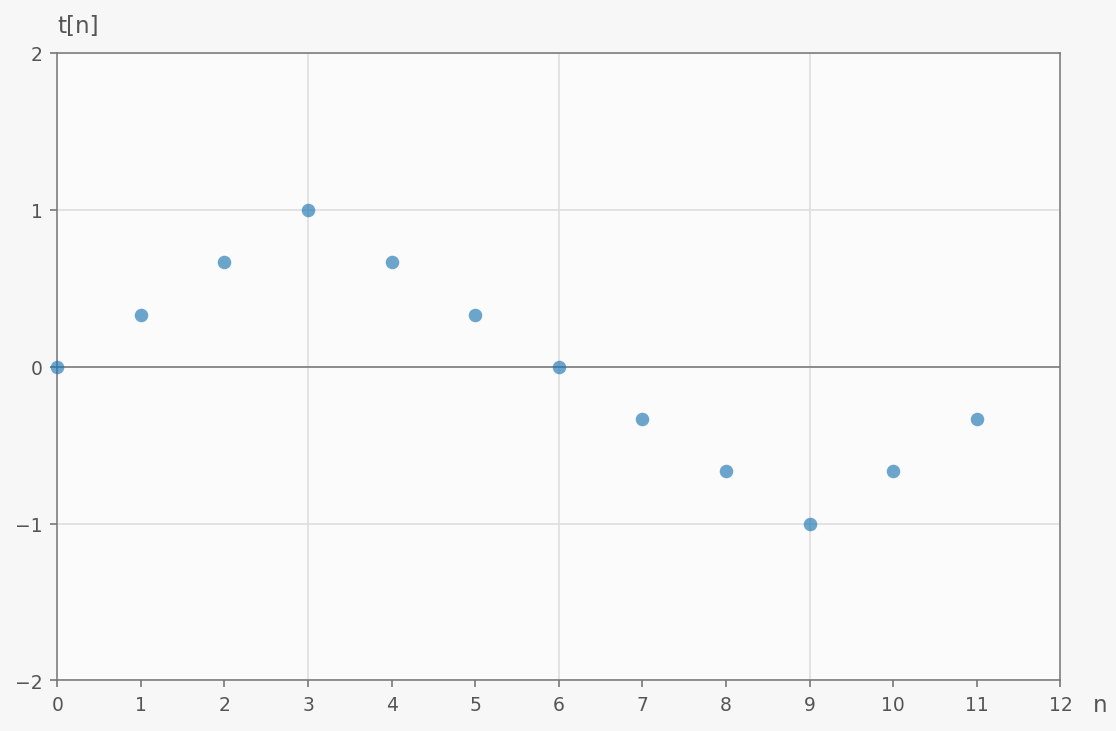
In code, the signal is an array of numbers:
x = np.array([0, 1, 2, 3, 2, 1, 0, -1, -2, -3, -2, -1]) / 3
The DFT of this signal produces complex coefficients, reported as magnitude–phase pairs. Phase is shown only for nonzero coefficients, since the phase of zero is undefined:
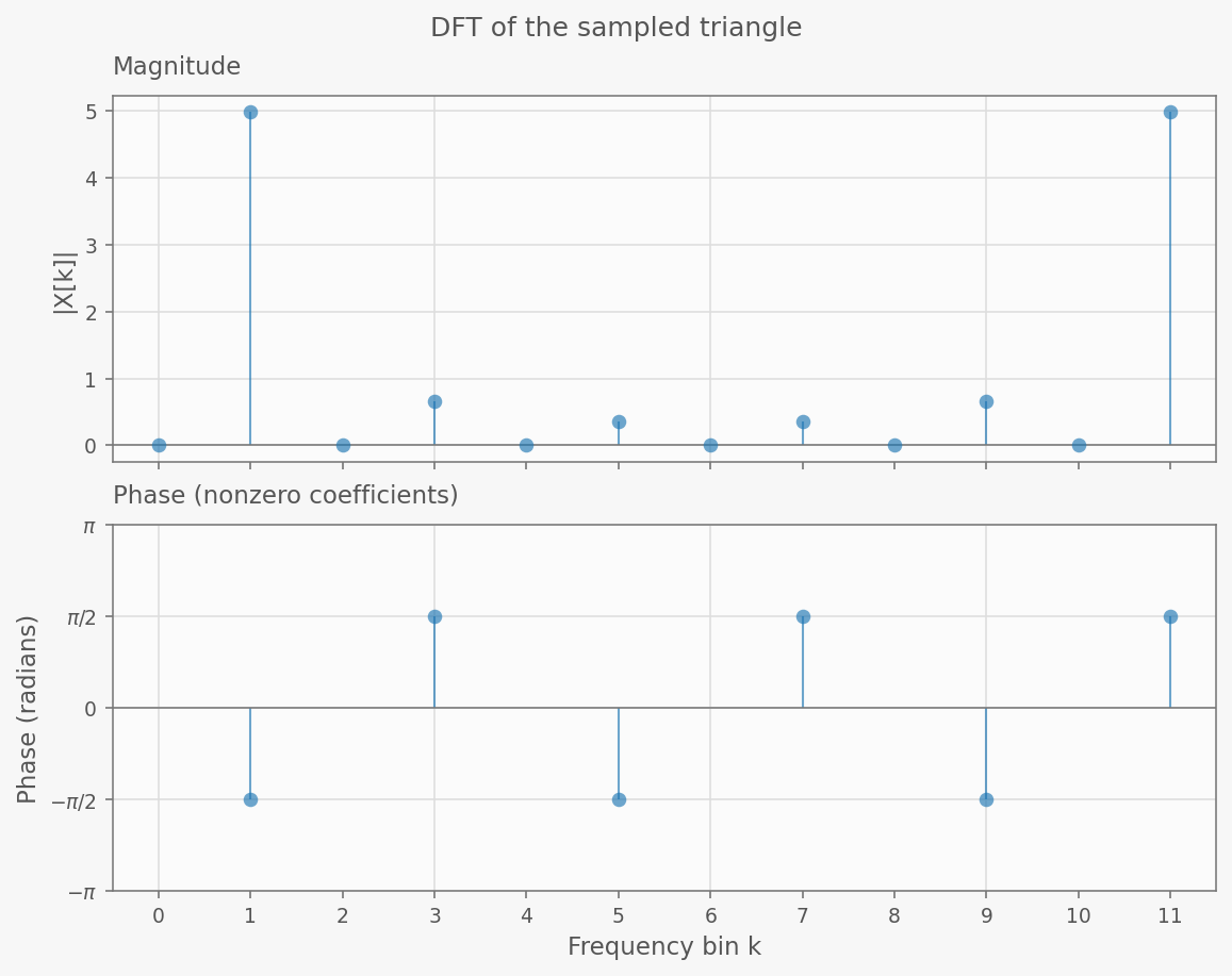
Matrix multiplication produces the same numbers. Multiplying by the computed IDFT matrix returns the original signal precisely, with differences attributable only to floating-point round-off.
Fast computation
The sample code also computes the same DFT with NumPy's fft.fft. This is the Fast Fourier Transform, an algorithm that exploits the structure of the Fourier matrix to compute the matrix–vector product in far fewer operations than direct multiplication. It is widely regarded as one of the most important algorithms of the 20th century; its inner workings are a subject for separate treatment.
Appendix: spectral leakage
The example above conveniently uses one full cycle of the triangle wave, so repeating the block reproduces the original waveform. If only part of a cycle is captured, naive periodic extension produces a jump at every cycle boundary. The DFT can still be computed, but the original triangle's frequencies no longer coincide with the DFT's frequency bins, so their contributions spread across multiple bins — spectral leakage. The coefficients still appear in conjugate pairs because the samples are real.
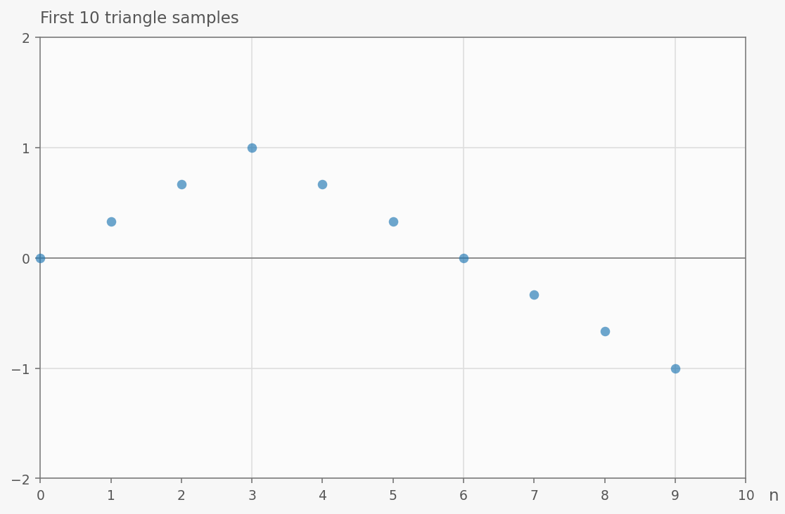
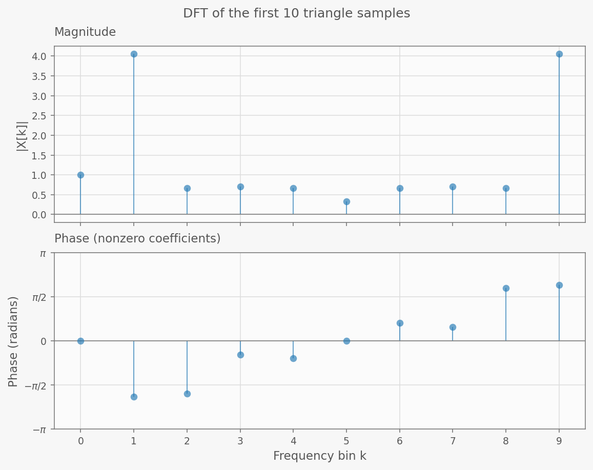
Applying the IDFT still reconstructs the short signal perfectly, so leakage is harmless when only reconstruction is needed. For frequency analysis it distorts the picture, adding frequencies that were not present in the underlying triangle wave in order to account for the discontinuity. Practical signal processing typically addresses this with window functions applied after sampling, which taper the signal toward zero at its edges and thereby reduce leakage.