What “Bayesian A/B Testing” Actually Means
Bayesian inference for A/B testing has become a standard feature in commercial experimentation platforms—GrowthBook, LaunchDarkly, PostHog, Amplitude Experiment, Optimizely, VWO, Statsig, and Eppo all ship a Bayesian mode. The pitch is usually that Bayesian statistics are modern, flexible, and easier to interpret than frequentist methods, and that complications such as multiple testing or sequential testing disappear naturally under the Bayesian framework.
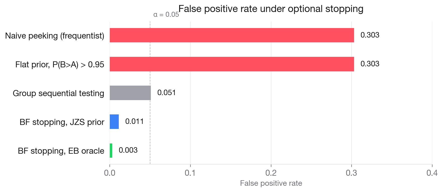
The reality is less tidy. Bayesian A/B testing is not a single method. It is a family of configurations—each defined by a stopping rule, a prior, and a likelihood. Depending on those choices, the result ranges from state-of-the-art sequential procedures to something numerically indistinguishable from peeking in a frequentist setting. Details matter, and the default configuration in most platforms is precisely the one that reproduces the false positive rate of naive frequentist peeking.
Start With Program Goals, Not the Tool
Companies running an experiment program should begin by asking what the program is supposed to achieve. Goals might include limiting the number of shipped features with no real effect, estimating impact with a specified precision, or minimizing some cost function over a sequence of experiments. The right statistical configuration depends entirely on these goals and constraints. There is no universally safe, model-agnostic default.
A Family of Configurations With Different Guarantees
Different Bayesian setups offer different protections, and they are not interchangeable:
- Flat prior with a posterior-probability stopping threshold—the default in almost every Bayesian-capable platform—reproduces the false positive rate of frequentist peeking.
- Bayes factor stopping compares evidence for a treatment effect against the null. Because the Bayes factor is a martingale under the null, thresholding it provides false positive rate control under optional stopping.
- Calibrated empirical Bayes priors can shrink effect estimates to counter winner’s curse bias and can bound the false discovery rate.
- Decision-theoretic approaches choose stopping rules that minimize a specified cost function. Whether they control frequentist error rates depends on how the problem is framed; sometimes they do, sometimes they do not.
These are not cosmetic variations. Each configuration has different guarantees and answers a different goal for the experiment program. The oversimplified Bayesian-versus-frequentist debate obscures this important distinction and often leads practitioners to adopt procedures with no better guarantees than the worst frequentist habits.
Bayesian and Frequentist Frameworks Overlap
Our recent paper on the topic reaches a central conclusion: the two frameworks are far closer than the debate suggests. In the paper, we:
- Examined generic claims about Bayesian A/B testing and identified exactly when—and under what conditions—they hold.
- Organized Bayesian configurations into tiers based on the guarantees they provide for an experiment program.
- Showed that Bayesian decision-theoretic formulations can be translated into equivalent frequentist formulations.
- Argued that Bayesian and frequentist experimentation cases overlap substantially in practice.
Why Spotify Sticks With Frequentist Tooling
Spotify’s current experimentation infrastructure is based on frequentist methods. Given the analysis above, adding a Bayesian inference mode would introduce a new set of configuration choices—prior, likelihood, stopping rule—each carrying its own error rate guarantees or lack thereof. None of this comes for free. The frequentist tooling already in place provides well-understood control over error rates, and a simple Bayesian layer on top would not automatically do better. In fact, without careful configuration, it would quite plausibly do worse. Until the Bayesian offering is capable of providing the same level of guarantee clarity that existing frequentist tools provide, there is no compelling reason to add it.
Goals vs. Configurations: The Real Source of Confusion
Much of the public debate around Bayesian A/B testing is muddled because it conflates two separate things: what an experimentation program wants to achieve (its goals) and the specific statistical setup it uses to get there (its configuration). A statement that sounds like a universal property of Bayesian inference is often true only for one particular pairing of a goal with a configuration. The key to making sense of the discourse is to separate those two layers.
It is also worth stating plainly: frequentist error rates are not a purely philosophical concern. Any experimentation program — Bayesian or otherwise — will accumulate false positives and false negatives over time. The real question is whether the program’s goals include controlling those rates, and whether its chosen configuration has the knobs to do so.
Peeking and the Likelihood Principle
The common claim that “Bayesian A/B testing does not require peeking correction” can mean two very different things. The first is that you do not care about the false positive rate under peeking — a statement about your goal. The second is that you are using a configuration, such as Bayes-factor stopping, that automatically keeps the false positive rate in check — a statement about your setup. Those are not the same argument, and treating them as one generic property of “Bayes” is what fuels the confusion.
The usual theoretical justification for ignoring the false positive rate is the Likelihood Principle: the posterior remains a valid belief update no matter when or why data collection stopped. That is correct, but it is a narrow guarantee. It says nothing about error-rate control, estimation precision, or decision-theoretic performance, all of which depend on the prior and the stopping rule. A coherent posterior is rarely the only thing an experimentation program cares about.
On the other hand, if your goal is to bound the false positive rate under peeking, Bayes-factor stopping is the natural Bayesian configuration for it. Crucially, the Likelihood Principle and false-positive control are not in tension; with Bayes-factor stopping you get both. Interestingly, no platform we are aware of currently offers Bayes-factor stopping as an option.
Decision theory offers a more formal route to the same conclusion. By encoding goals as cost functions and deriving the optimal stopping rule, you find that for several common cost functions the optimal rule is Bayes-factor stopping, which then bounds error rates indirectly. We will return to this point later.
Multiple Metrics Are Not Automatically Handled
Another common assertion is that “Bayesian testing handles multiple metrics automatically.” This hides how specific and demanding the relevant configuration really is. The claim is only true for a very particular setup, and it aims at a different error rate than most readers assume. There are two parts to this. First, what can be bounded without an explicit multiple-testing correction is the false discovery rate, not the false positive rate that most people would naturally think of. Second, the configuration that delivers that guarantee requires far more than a default Bayesian analysis: it requires Bayes-factor stopping together with a well-calibrated Empirical Bayes prior, fitted on a program's historical experiments.
That prior must include a point-mass component representing the historical fraction of null metrics. That component is what absorbs the multiplicity correction — it is not an absence of correction, but a sophisticated version of one. When the prior is well calibrated, this setup controls the false discovery rate across metrics. When it is poorly calibrated, the false positive rate is not bounded. And maintaining such a prior requires a continuously curated archive of past experiments, with no inappropriate pooling across heterogeneous programs or metrics, no undetected drift, and no selection bias in the corpus. Fail any of those conditions and the guarantees evaporate.
A more honest version of the claim would be: “If you have a well-calibrated empirical Bayes prior that applies to all metrics and you use Bayes-factor stopping, you can bound the false discovery rate without explicitly correcting for the number of metrics.”
The Winner’s Curse and Prior Shrinkage
The claim that “Bayes fixes the winner's curse” is the least problematic of the four, but it still needs qualification. Any informative prior shrinks the effect estimate toward its mean, and that shrinkage counteracts the winner's curse. With a reasonable informative prior, shipped effect estimates are less inflated than those from a flat prior or a frequentist point estimate.
The catch is that most teams running Bayesian A/B testing use the platform default, which is typically a flat prior. A flat prior provides no shrinkage — the posterior mean equals the maximum likelihood estimate, so the winner's curse is exactly as severe as in the frequentist case. The claim only holds for those using an informative prior, and the degree of correction depends entirely on the quality of that prior. A well-calibrated empirical Bayes prior goes further by adjusting shrinkage to the program's actual effect-size distribution: it shrinks toward the right target by the right amount.
In our simulations, a well-calibrated historical prior achieved the lowest estimation error of any configuration we tested. But a misspecified prior made things worse, not just comparable to having no prior — actively worse than baseline group sequential testing (GST). We tested two common failure modes: an archive containing only experiments that had already won, and a pool that mixed different programs. Both degraded estimation accuracy.
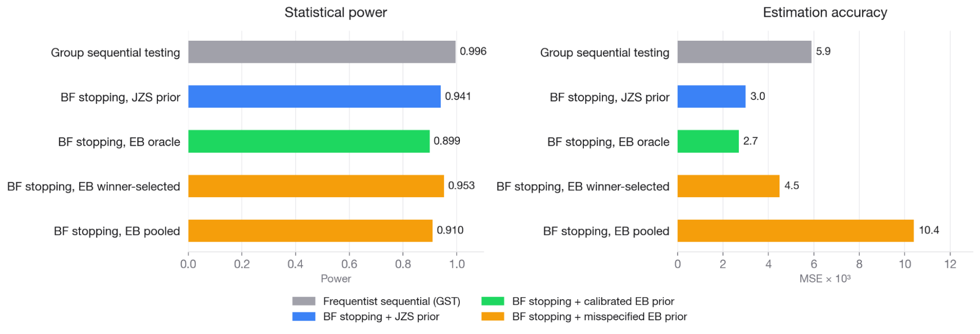
The takeaway: an informative prior clearly helps estimation accuracy, but incorrect pooling in a historical prior can make accuracy worse. And even with an oracle historical prior — the best possible prior for a given program — there was no power advantage over GST.
Practical Challenges of Empirical Bayes
Both of the previous sections point to the same conclusion: Bayes-factor stopping combined with a well-calibrated empirical Bayes prior offers genuine advantages that frequentist methods do not replicate as neatly. Estimating such a prior to sufficient quality is the hard part.
The corpus needs to be large — sometimes over 200 experiments — and representative. But even with enough experiments, prior estimation can fail in ways that more data will not fix. The most obvious trap is pooling across experiments that come from different treatment-effect distributions, or across metrics from the same program that behave differently. For example, a program tracking both sign-up rate and recommendation click-through rate might see the former barely move in most experiments while the latter shifts easily. Pooling both into one corpus makes the prior variance too wide for sign-up and too narrow for click-through, and skews the null-rate estimate because the two metrics have different true null rates. You end up with a prior calibrated to a distribution that neither metric actually follows.
Estimating one prior per metric solves that, but requires backfilling many historical experiments each time a new metric is introduced. There is also the underlying assumption that future experiments are exchangeable draws from the same distribution as past ones. Effect distributions change within a program over time — from diminishing returns and a changing world — which makes it genuinely hard to assess when historical data is representative of what is coming next.
Organizations with a single mature program, consistent metric definitions, and dedicated statisticians maintaining the prior can get real value from empirical Bayes. For most teams, the complexity of maintaining the prior will likely outweigh the benefits.
When Decision Theory and Error Rates Converge
The claim that “we need Bayes because we want to take a decision-theoretic approach” hides an important nuance. Decision theory itself is not inherently Bayesian, but in A/B testing the optimal policies turn out to be Bayes rules. For a simple and natural cost function that sums the costs of false positives, false negatives, and sampling, the optimal or near-optimal policy uses Bayes-factor thresholds. Because those thresholds also carry error-rate guarantees, the decision-theoretic and error-rate formulations become two parametrizations of the same kind of configuration. A frequentist choosing alpha and beta by thinking about costs has implicitly chosen a cost function. A Bayesian specifying costs inherits error rates.
The convergence does not hold for every cost function, and the exception is instructive. Expected-loss stopping, as described by Stucchio, triggers when the posterior is tight enough that the expected harm is small. Even under a true null effect, it will eventually ship the new variant once the posterior concentrates around zero. With a flat prior the false positive rate is around 50%, but if shipping a null effect is genuinely costless, that is the optimal stopping rule.
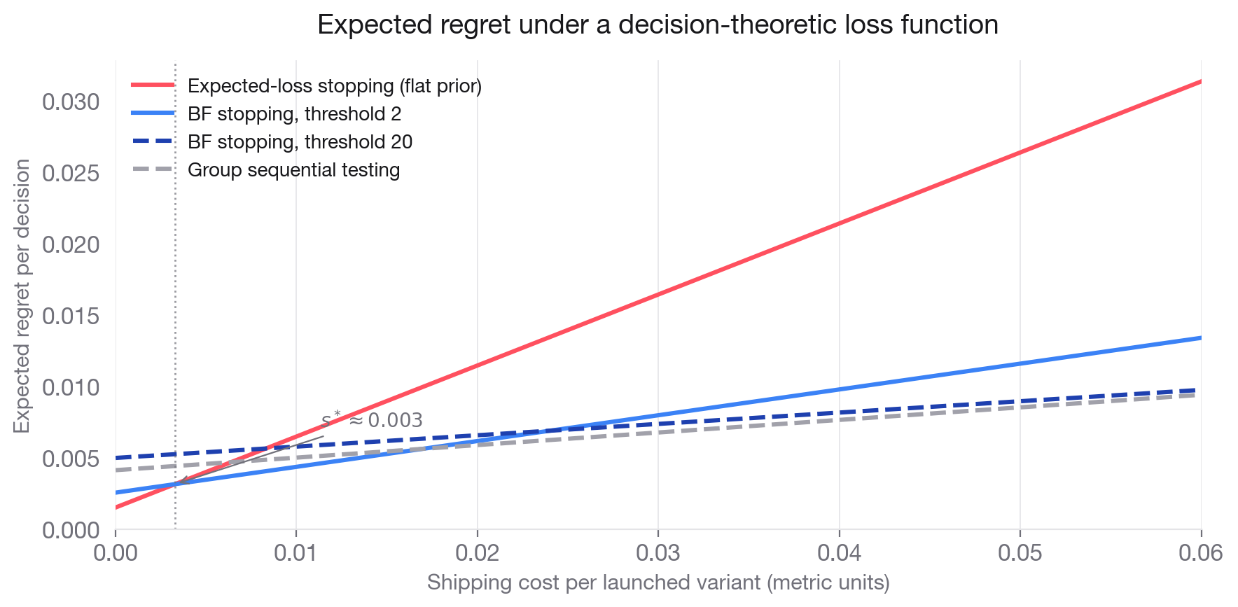
Once that shipping cost exceeds a few percent of a typical real effect, the rule is no longer optimal. So the right framework depends on what the cost function actually implies. For cost functions whose optimal policy is a Bayes-factor threshold, the decision-theoretic and error-rate views are two ways of describing the same rule — and many teams could capture most of the value by choosing their alpha and power based on a cost formulation, without switching frameworks. For cost functions whose optimal policy is not a Bayes-factor threshold, the decision-theoretic formulation genuinely diverges from error-rate control.
The Frameworks Are Closer Than the Debate Suggests
For the configurations most commonly deployed in practice, Bayesian and frequentist A/B testing are far more similar than the discourse implies. Under a flat prior and the two-group normal model, the outputs are numerically identical. The posterior mean equals the maximum likelihood estimate. The one-sided posterior probability that B beats A is one minus the p-value. A 95% posterior-probability threshold is algebraically equivalent to the one-sided frequentist rejection region. An experimenter running flat-prior Bayesian inference with posterior-probability thresholds is doing frequentist inference under a different vocabulary.
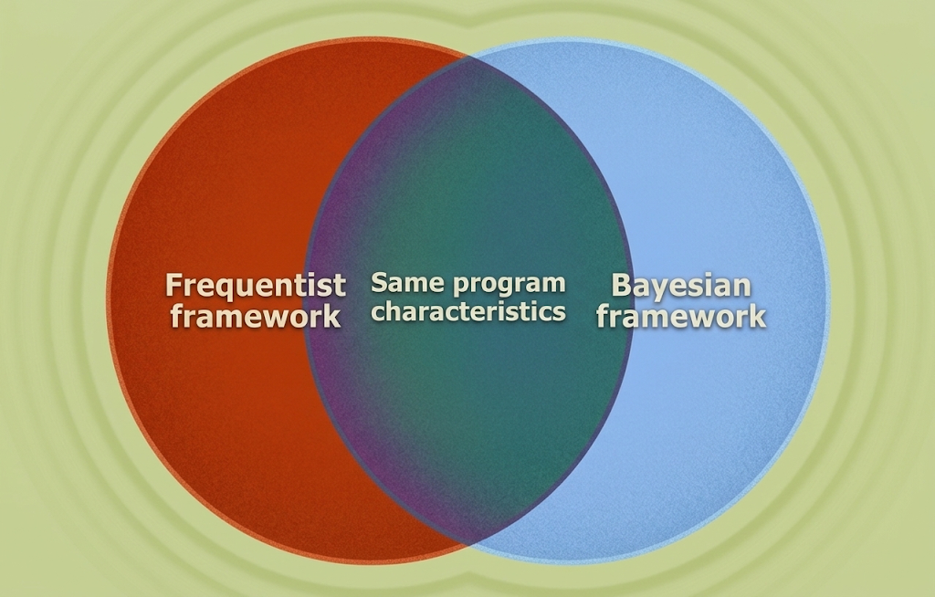
The connection runs deeper than the flat-prior case. The mixture Sequential Probability Ratio Test — one of the most well-known frequentist sequential procedures — is exactly the Bayes-factor stopping rule under the same prior. A frequentist who picks a mixing distribution to maximize power at the minimum detectable effect is, in Bayesian terms, placing a prior on the treatment effect. The mixing distribution is the prior.
The full picture then closes the loop. The optimal decision rule for many natural cost functions is a Bayes-factor threshold. That threshold is the mSPRT. The mSPRT is well approximated by group sequential testing (GST). There is a strong relationship between costs and error rates. A frequentist thinking in alpha and beta, or a Bayesian thinking in costs, very often lands on the same configuration. Frameworks are not opposites; the dominant configurations of each largely overlap in their guarantees.
Is the interpretability worth it?
A statement like “there is a 95% probability that the effect lies between 0.2% and 1.1%” is undeniably easier to communicate than a lesson in confidence intervals. But Spotify argues that this advantage is oversold.
With a flat prior, every Bayesian probabilistic statement maps one-to-one to a frequentist quantity. Point estimates and interval bounds are identical; the posterior probability that one variant beats another is simply one minus the p-value. A meaningfully different interpretation only emerges with a well-specified prior — and that prior is not free. It adds complexity in specification, justification, maintenance, and explanation. The framework trades interpretability for complexity elsewhere.
Bayesian methods do enable computation of richer quantities, such as the probability of exceeding a business threshold or of one variant being the best. These are genuine strengths, but it's unclear how often decisions actually change because such information is available. In practice, Spotify finds the interpretation debate less critical than it appears: they haven't seen product decisions deteriorate because someone treated a confidence interval as a probabilistic statement. What matters is that evidence is correctly propagated into decisions, not the technical purity of an intermediate step.
Why not both?
All of Spotify's production experiments currently run on frequentist statistics. The question of whether to add Bayesian modes — or switch entirely — has been debated internally at length. Spotify evaluates this against the core objectives of its experimentation program:
- Minimize experiments leading to poor business decisions (shipping harmful changes, or maintaining changes that don't improve user experience).
- Keep experimental evidence trusted.
- Make results hard to misinterpret, especially across teams and departments.
- Keep experiments easy to plan and configure, but hard to misconfigure.
Supporting two modes of inference would mean different planning, monitoring, interpretation, and output formats. Given Spotify's highly collaborative culture where people constantly set up and consume experiments company-wide, the cost of maintaining dual modes is high. The benefit of a second framework hasn't outweighed that cost.
Not every Bayesian setup would warrant this expense. One configuration Spotify identifies as genuinely advantageous would be a well-calibrated empirical Bayes prior for shrinkage and automatic FDR control. However, such a prior would need to be maintained at a high quality across every metric and program — and an incorrect prior can lead to poor decisions, eroding trust over time. This echoes a principle Spotify has written about before: sophistication that adds confusion can weaken evidence rather than strengthen it.
Spotify also contends that the framework debate absorbs energy better spent on fundamentals. Are decisions aligned with the inference being used? Does the sample size calculator match real decision rules? Are experiments generating learning rather than just ship decisions? Spotify has invested heavily in these integrations and observes that many companies debate Bayesian-versus-frequentist modes while still not nailing the basics of either. Flexibility tends to attract teams without full accounting for its complexity.
Spotify's closing advice: decide which guarantees you need and can consistently maintain, then weigh whether a specific Bayesian configuration meaningfully improves on the current framework. For Spotify, that improvement isn't there yet.