Choosing a Sequential Testing Framework — Comparisons and Discussions

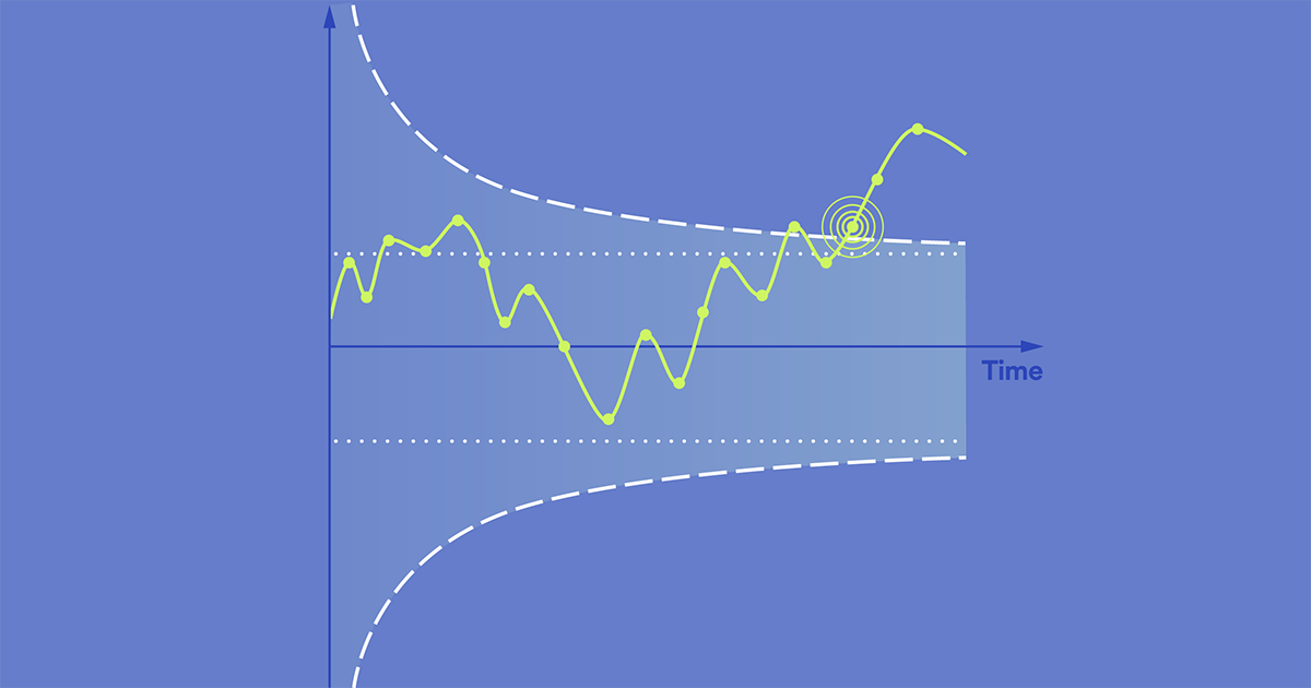
The core trade-off in sequential testing

Sequential testing has become the default for online experimentation, yet the literature offers surprisingly little guidance on which method to adopt. Most leading A/B testing platforms have their own preferred approach, and nearly all of them claim some form of optimality. The choice ultimately comes down to two practical constraints: whether your data pipeline delivers observations in streaming or in batches, and whether you can estimate the maximum sample size an experiment will reach before it starts.

Spotify's Experimentation Platform relies on group sequential tests (GSTs) with alpha spending as proposed by Lan and DeMets (1983). Simulation results show that when the maximum sample size can be estimated, GST delivers the highest statistical power whether data arrives continuously or in batches.

Why peeking breaks classical statistics

Experimentation platforms must guard against two types of product risk: shipping changes that hurt the user experience, and missing changes that would improve it. In statistical terms, these are false positives and false negatives. Standard tests like the z-test or t-test control these error rates only when applied once, after data collection is complete. Peeking — running the same test repeatedly during data collection — inflates the false positive rate because each additional test creates a new opportunity to stumble on a spurious effect.

Consider an experiment on 1,000 users split evenly between control and treatment. Applying a z-test after every new pair of observations and stopping only when a significant result appears yields an effective false positive rate that quickly exceeds the intended 5% — roughly 10% after just two tests. This is not a subtle degradation; repeated peeking can drive the true error rate to multiples of the target.

The landscape of sequential methods

Sequential tests allow repeated hypothesis testing during data collection without the error inflation that plagues naive peeking. They differ substantially in their requirements. Some require prior knowledge of the eventual sample size; others do not. Some suit streaming data, while others are designed for batch arrivals. We compare four families of methods, focusing on statistical power — the rate of rejecting the null hypothesis when a true effect exists.

The methods under consideration:

• Group sequential test (GST): used at Spotify with alpha spending.
• Mixture sequential probability ratio test (mSPRT): a special case of always valid inference popularized by Optimizely, Uber, Netflix, and Amplitude.
• Generalization of always valid inference (GAVI): proposed by Howard et al. (2021), used by Eppo.
• Corrected-alpha approach (CAA): proposed and used by Statsig.
• Bonferroni corrections: a conservative baseline that divides alpha by the number of peeks.

Group sequential tests

GSTs work as a series of traditional tests, exploiting the known correlation between intermittent analyses to allocate error probability optimally across peeks. The alpha-spending variant lets you distribute alpha arbitrarily over the timing of your peeks, and unused alpha carries over if you skip an analysis. If you never peek, the test reduces to a standard z-test at the end of the experiment.

Advantages:

• Alpha spending is flexible: you decide when to test and how much alpha to allocate to each look.
• Close to classical z-test intuition, making it easy to explain to experimenters.

Disadvantages:

• Requires a reliable estimate of the maximum sample size. Undershooting makes the test conservative; overshooting inflates the false positive rate.
• Under-observation can make the choice of spending function materially affect power.
• Critical values require numerical integration, which limits GSTs to at most a few hundred intermittent analyses — not feasible for true streaming.

Always valid inference

AVI methods (mSPRT and GAVI) permit continuous testing with no pre-declared stopping rule or sample size bound. They are simple to implement and support both streaming and batched data, but they require choosing a mixing distribution — the distribution of the effect under the alternative hypothesis. That choice materially affects test properties, and if the expected sample size is used to guide the choice, the advantage of not needing a sample size estimate evaporates.

These tests are also harder for practitioners trained in traditional hypothesis testing, and they exhibit lower power by construction when data arrives in batches rather than streams.

Conservative baselines

Bonferroni corrections provide a straightforward safeguard when you can bound the number of peeks: use z-tests with alpha divided by that maximum count. The method is easy to implement and explain, but the test statistic's high correlation across peeks makes it unnecessarily conservative, and power degrades quickly as the number of intermittent analyses grows.

The corrected-alpha approach used by Statsig takes a different route: it accepts some false positive inflation in exchange for a simple adjustment. This caps the damage but does not bound the error rate at the intended alpha level. The true false positive rate depends on the sample size and the timing of peeks, which complicates interpretation even if the method is easy to apply.

What this means for your platform

The deciding factors are practical. If your infrastructure delivers data daily or at other batch intervals and you can estimate the experiment's maximum sample size with reasonable confidence — as is typical when traffic is predictable — GST with alpha spending gives you the highest power. If you cannot estimate the sample size or need unlimited, continuous testing, always valid inference methods become attractive despite their parameter-tuning burden. Bonferroni and other conservative fixes are workable only when the number of peeks is small and power loss is acceptable.

The simulation evidence reinforces that context matters more than any single method's theoretical guarantees. The right choice follows from the structure of your data pipeline and your ability to forecast experiment traffic.

Batch versus streaming data

How results are delivered often dictates which sequential testing approach is practical. With batch data, analysis can happen no more often than each new batch arrives. Spotify, for instance, runs most data jobs daily, giving one analysis opportunity per day during an experiment. The group sequential test (GST) is built for exactly this pattern of intermittent batch analyses. Its main limitation is numerical: if the number of interim analyses exceeds a few hundred, the required integrations become intractable. Since most Spotify experiments run for a few weeks at most and receive data in daily batches, the GST fits the environment well.

Streaming data, by contrast, admits an analysis after every new observation. The always-valid inference (AVI) family — GAVI and mSPRT — can compute as soon as a new observation arrives, and ideally should be used this way to reach significance quickly. These tests can still handle batch data by skipping interim analyses, but doing so makes them conservative because many chances for false positives are never considered. This point returns in the simulation results below.

What matters when comparing tests

Two properties dominate practical assessments of sequential tests:

• Bounded false positive rate: The test must control the false positive rate at or below the intended alpha even when experimenters peek at results repeatedly.
• Power: The test should reject the null frequently when a true effect exists.

Other dimensions — supported test statistics, small-sample behavior — matter, but power and false positive control are the most consequential starting points. Of the five tests discussed, all but the corrected-alpha approach (CAA) bound the false positive rate under peeking. CAA spends its full alpha budget only at the final analysis; any peeking before that inflates the overall rate, with the degree of inflation depending on how often and how much data is examined. Because CAA fails the first criterion, it is excluded from power comparisons.

Simulation setup

A Monte Carlo study illustrates the trade-offs. Data is generated from a normal distribution with mean 1 (plus a treatment effect under treatment) and variance 1. Sample sizes are balanced at 500 per group. Each setting runs 100,000 replications with one-sided tests at alpha = 5%. The number of evenly spaced interim analyses varies: 14, 28, 42, 56, or streaming (500 analyses in this setup). Streaming is not computed for the GST because it is impractical at typical online-experiment sample sizes.

GST bounds use the ldbounds R package with varying expected sample size [n]. GAVI follows Eppo’s documentation with the tuning parameter numerator [rho] varied. mSPRT uses the generalization by Lindon et al. (2022), restricted to one dimension, with tuning parameter [phi] varied. CAA follows Statsig’s documentation.

False positive rates

The empirical false positive rate simulation includes these variants:

• GST with correctly assumed sample size, 50% underestimated sample size, and 50% overestimated sample size. Oversampling applies the correction from Wassmer and Brannath (2016), pages 78–79. Two power-family alpha spending functions are used, quadratic and cubic in the information ratio, per Lan and DeMets (1983).
• GAVI with the tuning parameter numerator set to the correct expected sample size, and to 50% oversampled or undersampled values.
• mSPRT with [phi] equal to 1/[tau]^2, where [tau] takes one of the true effect sizes (0.1, 0.2, or 0.3).
• CAA with no settings.
• Naive Bonferroni-corrected z-tests with alpha divided by the number of interim analyses.

Table 1 shows results across the replications. Every test bounds the false positive rate except the oversampled GST and CAA. For the oversampled GST this is expected: all alpha is consumed once the planned sample size is reached, so tests beyond that point inflate the rate. CAA behaves symmetrically — it exhausts alpha only on the final look.

The always-valid tests (GAVI and mSPRT) are conservative when not run after every observation. Interestingly, the naive Bonferroni approach at 14 interim analyses matches some always-valid variants in conservativeness.

Power comparison

Methods that fail to bound the false positive rate are dropped from the power analysis. True effects of 0.0, 0.1, 0.2, 0.3, or 0.4 standard deviations are added; the zero-effect row corresponds to the empirical false positive rate. Table 2 reports power for a 0.2 standard deviation effect, chosen because no method saturates at power 1 or 0 at that size.

The GST dominates in most settings, even with overestimated expected sample sizes. The exception occurs when the alpha spending function spends little alpha early and the sample size is overestimated — then most of the budget is planned for a phase that never arrives. In that case GST power aligns with the always-valid tests but falls below the best always-valid variants.

The number of interim analyses barely affects GST power. For GAVI and mSPRT, fewer analyses reduce power, as expected. The differences are modest, but the naive Bonferroni test at 14 analyses outperforms all always-valid variants tested at that frequency. mSPRT and GAVI power remain relatively stable across tuning parameter choices.

Figure 2 shows full power curves for a subset of settings. Most variants perform comparably, with the main exceptions being GST and streaming Bonferroni. Bonferroni with 14 or 56 analyses does surprisingly well, but overcorrects badly at 500 analyses.

Practical takeaways

The GST is systematically better than or comparable to always-valid approaches. At Spotify, where data arrives in daily batches, the GST’s inability to handle streaming data is irrelevant — it is a feature, not a limitation. A more surprising result is that simple Bonferroni corrections on standard z-tests match always-valid tests when interim analyses are few. Always-valid methods may be overly conservative for many real settings.

These findings come from a deliberately simple simulation and may not generalize. The setup assumes an upper bound on sample size or experiment duration, which suits online experiments with planned stopping. For experiments that run indefinitely, always-valid tests become more attractive. The simulation also assumes known variance and normally distributed data; real-world violations could shift results for different tests in different ways.

Always-valid approaches require tuning parameters just as the GST needs an expected sample size. The key difference: any tuning parameter value for GAVI or mSPRT still guarantees the false positive rate never exceeds alpha — a poor choice only costs power. For the GST, underestimating the expected sample size inflates the false positive rate. If estimating the final sample size is hard and often wrong, the always-valid guarantee may be worth the power loss.

Severe Sample-Size Misspecification

The simulation results so far show that group sequential tests (GSTs) generally win on power when the expected sample size is known or can be estimated with reasonable accuracy. That assumption does not always hold — historical data may be unavailable for the type of experiment being run, making it impossible to forecast how many observations will be collected.

In that scenario, the always valid inference (AVI) family becomes more attractive. The simulations indicate that the number of intermittent analyses matters far less than the ability to estimate the expected sample size (for GST) or select the mixing parameter (for mSPRT and GAVI). Since the two AVI variants are comparable in power, the analysis focuses on GAVI, whose parameterized expected sample size makes reasoning simpler.

When using GAVI, underestimating the sample size used to select the mixing parameter is safer than overestimating it, per Howard et al. (2021). But if you have accurate sample-size information, GST is the better instrument. That makes GAVI most appealing precisely when sample size is hard to predict and you choose to underestimate it as a robustness strategy. The question is how much power GAVI sacrifices under severe underestimation.

To test this, a simulation optimizes GAVI for n=10 while the actual sample size reaches 500 — a 50-fold underestimate. To put that in context, Eppo currently uses n=10,000 as the GAVI setting for all of its sequential tests, so this scenario is equivalent to someone running a 500,000-user experiment with Eppo's configuration.

Table 3 reports empirical power across 100,000 Monte Carlo replications under a fixed treatment effect of 0.2 standard deviations, comparing GAVI with the 50-fold underestimated mixing parameter, GAVI with the correct sample size, GST with the correct sample size, and a Bonferroni correction. The GST uses a quadratic alpha spending function, the best performer from the earlier comparison.

The power loss from the 50-fold underestimation is roughly 15% relative to GAVI with the correct sample size, and about 30% relative to GST with the correct sample size. That 30% gap underscores how much accurate sample-size forecasting matters for achieving high power in sequential testing. Given that GAVI permits arbitrarily large samples, losing only this much power under such extreme misspecification is notable. Still, the Bonferroni approach outperforms GAVI in power for up to 56 preplanned intermittent analyses.

Choosing a Sequential Test in Practice

Always valid inference is attractive for experimenters new to sequential testing who mainly want bounded false positive rates and an early warning system. More sophisticated teams chasing power — for instance, those combining sequential tests with variance reduction — should be cautious: the power lost to AVI can offset the gains from standard variance-reduction techniques.

• When sample size cannot be estimated: AVI tests are a solid choice if data arrives as a stream. If data cannot be streamed, Bonferroni is a viable alternative provided the maximum number of intermittent analyses is fixed in advance.
• When sample size is estimable but overrunning may be needed: AVI remains usable, but it forfeits power compared to GST. Running longer than the estimated n can recover that loss, but only once the additional observations make up for the deficit.
• When early detection of large regressions is the priority: AVI works well on streaming data; neither GST nor Bonferroni can analyze a true stream. For large effects, power is not the limiting factor. For small regressions, batching with GST may detect deterioration earlier at comparable sample sizes.
• When sample size is estimable and overrunning is not required: GST is the recommended path, whether data is analyzed in batches or streamed through batching. To catch regressions early, schedule many intermittent analyses near the start. If you intentionally underestimate the expected sample size to avoid oversampling, avoid an alpha spending function that is overly conservative in early data collection.
• On GST flexibility: A common misconception is that GST requires the number and timing of intermittent analyses to be fixed in advance. Per Jennison and Turnbull (2000), you can conduct as many or as few analyses as you like at any point during data collection, paying only for the peeking that actually occurs.

Variance reduction note: All tests discussed here can be combined with linear-regression-based variance reduction. Because that technique can be implemented in two steps, residualization can be performed before applying any of the methods. Formal treatments exist for both AVI (Lindon et al., 2022) and GST (Jennison and Turnbull, 2000), so the relative comparisons in this analysis hold under the most common variance-reduction approach.

A Practical Perspective from Spotify

Spotify's Experimentation Platform relies on group sequential tests, a legacy of their origin in medical trials where data arrives in batches — mirroring the batch-oriented data infrastructure behind the platform. The simulation study confirms that even with streaming data available, analyzing in batches with GST yields a higher probability of detecting a real effect than streaming analysis with either AVI test.

The choice of test matters less than using one at all. Spotify's platform depends on sequential testing to let developers monitor experiments continuously and spot adverse effects quickly without inflating false positive rates. Any of the frameworks discussed here supports that capability; the decision among them should rest on data infrastructure, sample-size predictability, and the priority placed on raw power.