Series Forecasting with Recurrent Neural Networks (LSTM)

Setting Up an LSTM for Series Prediction

Recurrent neural networks have a well-deserved reputation for being finicky to work with. The Long Short Term Memory (LSTM) variant solves the vanishing/exploding gradient problem by keeping an internal state that carries information across many time steps. While the theory is well documented, practical examples are often muddled. Here, we build a working stateful LSTM with Keras to forecast monthly U.S. industrial production of electric and gas utilities from 1985–2018 (397 data points, available from the Federal Reserve or Kaggle).

Start by importing the necessary libraries and loading the data into a NumPy array:

from __future__ import print_function
import numpy as np
import matplotlib.pyplot as plt
import pandas as pd
from keras.models import Sequential
from keras.layers import Dense, LSTM

# Read data
raw_data = pd.read_csv('./Electric_Production_full.csv')
arr_data = np.array(raw_data.Value)

# Plot raw data
plt.plot(arr_data,label = 'Data')
plt.xlabel('time (months)')
plt.ylabel('Energy (au)')
plt.legend()
plt.savefig('data.eps', bbox_inches='tight',format='eps')
plt.show()

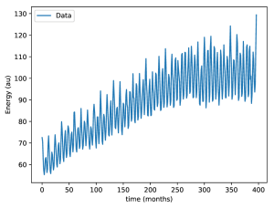
If imports fail, install Keras, TensorFlow, Pandas, NumPy, and Matplotlib.

Preparing Training and Test Windows

The key hyperparameter is lahead. It sets the explicit input window size. Here we use lahead = 1, meaning each prediction is based on exactly one data point. The LSTM's hidden state supplies the memory of everything seen before, which is why this works despite the series' complexity. More explicit history can be fed by raising lahead, but the stateful mechanism is what enables long-range dependence.

Of the 397 points, 270 go to training and the rest to validation. Standard univariate forecasting practice shifts the target by one step: training input x_train is the series up to position 269, and target y_train is the same series shifted by one. The arrays are reshaped to the 3D format Keras expects for LSTM layers.

# Set parameters
n_train = 270
lahead = 1 # time steps that the model incorporates explicitly in the input
# training parameters passed to 'model.fit(...)'
batch_size = 1
epochs = 600

# Split train and validation
n_data = arr_data.shape[0]
n_valid = n_data - n_train
arr_train = arr_data[:n_train]
arr_valid = arr_data[n_train:]

# split into input and target
x_data = arr_train[:n_train-1]
y_data = arr_train[1:] # same as x_data, but with lag

reshape_3 = lambda x: x.reshape((x.shape[0], 1, 1))
x_train = reshape_3(x_data)
x_test = reshape_3(arr_valid[:-1])
reshape_2 = lambda x: x.reshape((x.shape[0], 1))
y_train = reshape_2(y_data)
y_test = reshape_2(arr_valid[1:])

Validation is split the same way so the model sees the same one-step-ahead task during evaluation.

Architecture and Stateful Training

The network is deliberately small: one LSTM cell with 20 outputs feeding a single dense unit for the scalar prediction. The critical detail is stateful=True. Without it, Keras resets the LSTM's hidden state after every batch, and the memory mechanism is defeated. With it, state carries across batches within an epoch.

model = Sequential()
model.add(LSTM(20, input_shape=(lahead, 1), batch_size=batch_size,stateful=True))
model.add(Dense(1))
model.compile(loss='mse', optimizer='adam')
model_stateful = model

Training runs as a manual loop over epochs. Because the model is stateful, state must be cleared explicitly between epochs; an inner epochs=1 call with shuffle=False preserves temporal order. Mixing the loop with validation on the unseen test set lets us watch generalization without ever shuffling the series.

for i in range(epochs):
    print('iteration', i + 1, ' of ', epochs)
    model_stateful.fit(x_train, y_train, batch_size=batch_size, epochs=1,  validation_data=(x_test, y_test),  shuffle=False)
    model_stateful.reset_states()

Forecasting and the Role of Persistent State

After training, the state is reset. The training set is passed through the model once to prime its internal memory. Then the test set is predicted point-by-point, passing each value as a single input to the next step. Explicitly looping over test inputs demonstrates that each forecast depends on only the immediate prior observation plus whatever the cell has stored internally.

#Predict training values
predicted_stateful_train = model_stateful.predict(x_train, batch_size=batch_size)

#Predict test values one by one:
pred_test = []
for i in range(x_test.shape[0]):
    # Note that only one value x_test[i] is passed as input to the model to make a prediction!
    pred_test.append(model_stateful.predict(x_test[i].reshape(1,1,1), batch_size=batch_size))

#Convert list to numpy array
pred_test_1 = np.array(pred_test)

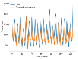
Plotting the one-step forecasts against actual values shows close alignment, even for a model whose explicit input is a single time point. That fit comes from the LSTM's memory, not from a wide context window.

#Plot
plt.plot(y_test.reshape(-1),label= 'Data')
plt.plot(pred_test_1.reshape(-1),label= 'Forecast one-by-one')
plt.xlabel('time (months)')
plt.ylabel('Energy (au)')
plt.legend()
plt.show()

What Happens Without a Primed State?

To see how much the internal state matters, reset the model and start predicting on the test set directly, without first feeding any training data. The reset wipes out all accumulated memory, so the first forecasts have no context to work with.

model_stateful.reset_states()
# Make predictions after model reset
pred_test_0 = []
for i in range(x_test.shape[0]):
    pred_test_0.append(model_stateful.predict(x_test[i].reshape(1,1,1), batch_size=batch_size))

pred_test_0 = np.array(pred_test_0)

plt.plot(y_test.reshape(-1),label= 'Data')
plt.plot(y_test.reshape(-1),label= 'Data')
plt.plot(pred_test_1.reshape(-1),label= 'Forecast')
plt.plot(pred_test_0.reshape(-1),label= 'Forecast reset')
plt.xlabel('time (months)')
plt.ylabel('Energy (au)')
plt.legend()
plt.show()

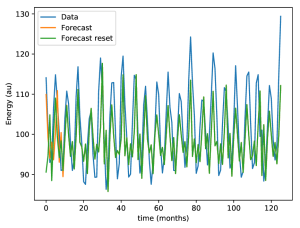
The contrast is instructive. The reset model (green) forecasts poorly in the beginning because its internal state is empty—it lacks the historical sequence needed to predict the next value. Once it ingests a few test points, its state populates and the forecasts converge to look like those of the properly primed model (orange). The persistent-state LSTM is doing exactly what it was designed to do: turning a bare time series into context for each subsequent prediction.