Bandwidth estimation meets machine learning
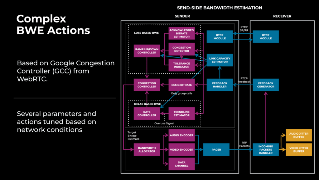
Meta’s real-time communication (RTC) stack originally leaned on WebRTC’s Google Congestion Controller (GCC) for bandwidth estimation (BWE). Years of parameter tuning kept the module working, but the cost was complexity: a tangle of conditions and branches that depended on specific network states. Engineers faced a constant trade-off between quality for high-bandwidth users and reliability for low-bandwidth ones; tuning for one often regressed the other. The iterative process was also slow — realistic network conditions were hard to reproduce during experimentation, and after rollout there was no certainty that the tuned parameters still matched the target network types.
To escape this tangle, Meta turned to machine learning. Instead of hand-tuned rules, the team built a model-based system that characterizes a network during a call, applies configuration parameters tuned offline for that network type, and allows updates in real time. The approach treats networking problems holistically, spanning BWE, network resiliency, and transport.
How network characterization works
For an RTC call to succeed, endpoints must connect through network devices. In Meta’s design, optimal configurations tuned from offline simulations are stored on a server and can be updated in real time. During call setup, the server sends the client the config that best matches the network type identified from collected signals. Media then flows directly between endpoints or through a relay, while ML characterizes the network during the call and applies the stored config appropriate to that type.
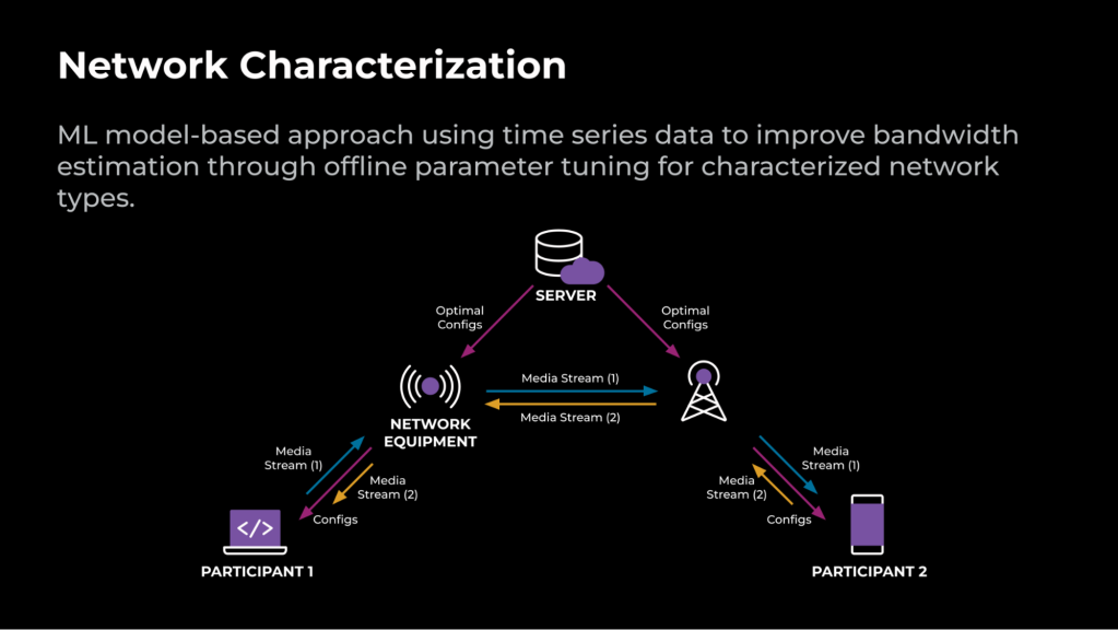
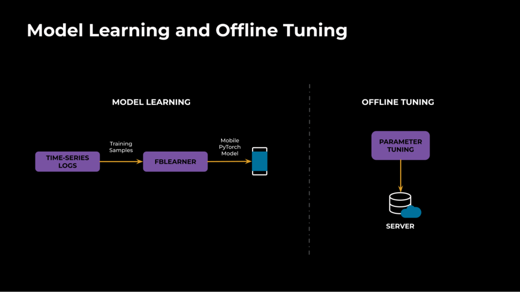
Network characterization has two pillars: offline model learning and offline parameter tuning. The first uses ML to categorize a network (for example, random packet loss versus bursty loss). The second runs simulations across network profiles for each detected type, picking parameters that maximize technical metrics such as quality and freeze rate.
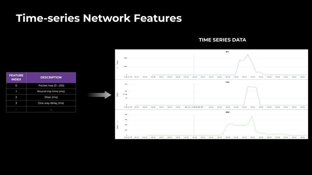
Feature engineering for these models captures two complementary signal categories:
- Time series data showing how network conditions evolve during a call.
- Non-time series, derived metrics computed from those time windows.
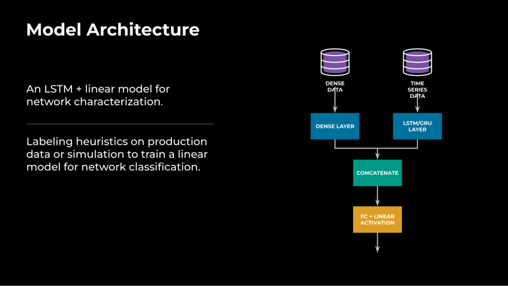
The time series data feeds an LSTM layer that compresses it into a one-dimensional vector (for instance, 16×1). Dense data passes through a fully connected layer. The two vectors are concatenated and fed through another fully connected layer, producing the model’s prediction.
Model training uses time series logs from production calls and simulations, containing network signals and non-personally identifiable information. FBLearner, Meta’s internal AI stack, handles the training pipeline; the resulting PyTorch model files are delivered on demand to clients at the start of a call.
Case study: Classifying packet loss
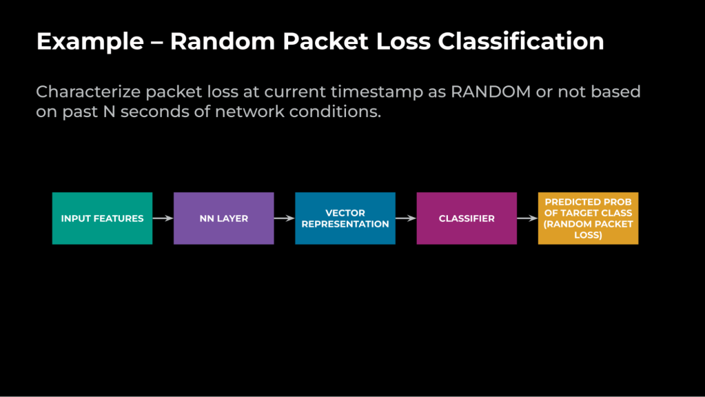
A concrete use case is telling random packet loss from congestion-induced loss. Random loss stems from network components; loss generated by congestion has queue length and delay fingerprints. The ML task is scoped as:
Given network conditions from the past N seconds (10), and evidence that the network is currently losing packets, classify those losses as random or not at the current timestamp.
When the model flags random loss, the BWE module takes local actions:
- Raise tolerance to random packet loss in the loss-based bitrate estimator, holding the current bitrate.
- Increase ramp-up speed on high-capacity links. When random loss is mistaken for congestion, the sender backs off unnecessarily; faster ramp-up after recovery limits the damage.
- Strengthen network resiliency by sending extra forward-error correction packets to cover random losses.
From classification to prediction
Classifying network types from past data with hand-tuned rules works to a point, but the real leverage of ML comes from forecasting network state. A first target: congestion prediction for low-bandwidth users, a population that per Meta’s production analysis frequently suffers congestion because of GCC’s behavior.
The problem definition uses round-trip time (RTT) and packet loss history to predict an imminent congestion event:
Based on time-series data from production or simulation over the past N seconds, predict whether congestion—manifested as an RTT spike eventually followed by packet loss or further RTT growth—will occur in the next N seconds.
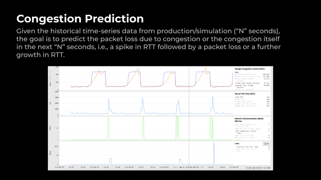
The value of predicting vs. reacting is visible in simulation: a link alternating between 500 Kbps and 100 Kbps every 30 seconds triggers congestion-clamped predictions just before the delay spikes and packet loss materialize. Reacting earlier reduces video freezes and connection drops.
Labelling congestion samples
The tricky part of supervised learning here is generating labels that reflect real-world congestion. Simulations can’t reproduce everything a production client experiences, so Meta pulled actual production logs and labeled congestion using RTT-spike criteria in past and future windows. Two assumptions drove the labeling:
- Packet losses in the past and future are independent if no RTT spikes appear in the past window.
- Future RTT spikes or fractional losses cannot be predicted if no RTT spikes appeared in the recent past.
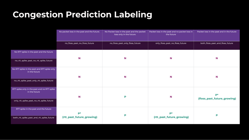
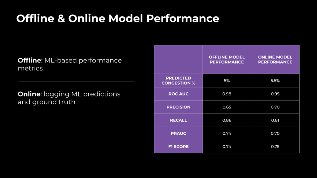
An eight-second window split was used for labeling — four seconds of history, four seconds of horizon. Unlike network characterization (where ground truth is unavailable), the future window offers it: predictions made four seconds earlier can be checked against subsequent logs. This offline-to-online consistency check is reflected in the deployment numbers.
Deployment results
Measurements from production clients show improvement across three applied models:
Congestion prediction improves reliability
- connection_drop_rate —0.326 +/- 0.216
- last_minute_quality_regression_v1 —0.422 +/- 0.206
- last_minute_quality_regression_v2 —0.371 +/- 0.196
- bad_experience_percentage —0.230 +/- 0.148
- transport_not_ready_pct —0.437 +/- 0.401
- peer_video_freeze_percentage —0.749 +/- 0.181
- peer_video_freeze_percentage_above_500ms —0.439 +/- 0.212
High-bandwidth random loss classification boosts quality
- peer_video_freeze_percentage —0.379 +/- 0.125
- peer_video_freeze_percentage_above_500ms —0.542 +/- 0.141
- peer_neteq_plc_cng_perc —0.242 +/- 0.137
- total_talk_time +0.154 +/- 0.149
Cellular low-bandwidth classification helps reliability and quality
- connection_drop_rate —0.196 +/- 0.128
- last_minute_quality_regression_v1 —0.199 +/- 0.125
- last_minute_quality_regression_v2 —0.188 +/- 0.138
- peer_neteq_plc_cng_perc —0.360 +/- 0.192
- peer_video_freeze_percentage —0.653 +/- 0.143
Cellular high-bandwidth classification lifts both quality and reliability
- avg_sender_video_encode_fps +0.152 +/- 0.047
- avg_sender_video_qp —0.228 +/- 0.042
- avg_video_quality_score +0.297 +/- 0.043
- avg_video_sent_bitrate +0.430 +/- 0.092
Consolidating future work
Meta sees ML not as a drop-in replacement for heuristics but as a way to target, monitor, and update the congestion control behavior more cleanly. Work so far has focused on classification and prediction; the team plans to consolidate the separate network-characterization models into a single multi-task model. Features:
- A shared time-series representation for different tasks — bandwidth classification, packet-loss type, etc.
- More realistic production-network scenarios fed into training and validation, allowing model-driven decisions about optimal network actions, not just picks among hand-set config parameters.
- Ongoing refinement of learning-based methods given the existing network signals.