Why pairwise demand forecasts are failing us
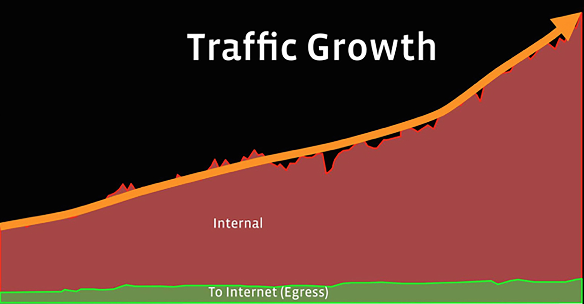
Meta’s production backbone carries traffic between data centers and out to users, with demand patterns shifting constantly as services evolve, new workloads appear, and user behavior changes. The result has been years of exponential growth and highly variable traffic demand. Keeping up with that demand has traditionally meant predicting the full future traffic matrix: the pairwise volume between every pair of data centers. That forecast is central to capacity planning, but it’s also fundamentally fragile.
The classical planning approach sizes the topology around a forecast traffic matrix, under a defined failure protection policy covering events like single fiber cuts or dual submarine link failures. A cost optimization model, typically an integer linear programming formulation, then computes the capacity plan that keeps the traffic flowing under all failure scenarios in the policy.
Several problems pushed us to abandon this model:
- Long lead times, poor long-term fidelity: Backbone capacity turnup takes months or years, particularly when it involves building terrestrial fiber routes or submarine cables. Service behavior over that timescale is hard to predict, and services themselves change constantly. Asking every service owner to give an explicit demand spec per data center pair is unmanageable; new services and even new data centers may not exist at forecast time. Historically, uncertainty was absorbed by over-provisioning to a high percentile, like P95.
- The network isn’t a consumable resource: Services can reason about compute and storage as finite resources per data center, but the network is shared and opaque. A planning method should abstract the network so services can treat it like any other per-data-center resource.
- Operational churn: Tracking every service’s traffic surge, root-causing it, and estimating impact creates overhead. Most surges are harmless because not all services peak simultaneously, but each one still generates false alarms and toil.
The network-hose model
Instead of forecasting pairwise traffic, we now forecast total egress and total ingress per data center: the network hose. The question changes from “how much traffic will a service send from X to Y” to “how much ingress and egress traffic will a service generate at X.” This replaces O(N^2) data points per service with O(N), and the aggregated forecast naturally incorporates statistical multiplexing.
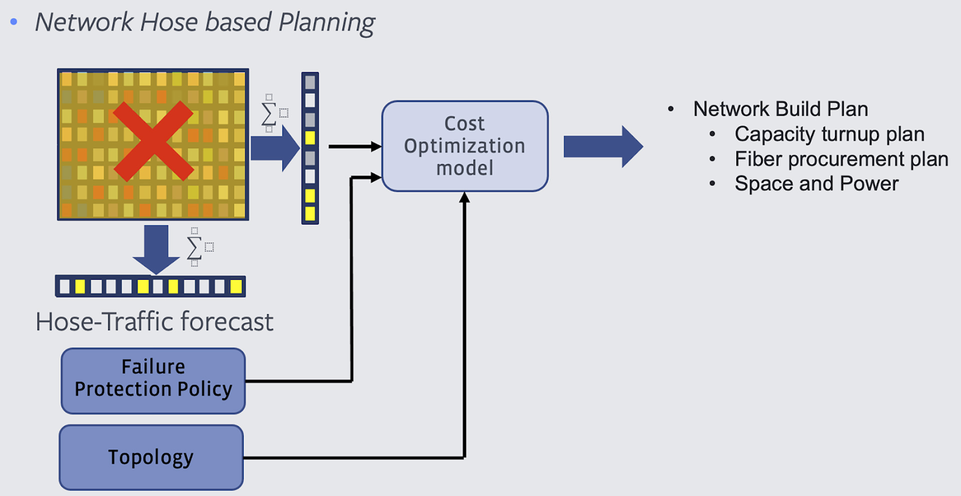
This is a simpler, coarser planning signal, but it introduces its own challenge. The hose constraint defines a convex polytope of all possible demand sets that could satisfy it. A single point inside that polytope is one full traffic matrix; a long-term plan that must satisfy the hose constraint has to accommodate all demand sets in that space. Since designing a cross-layer global production network for even one demand set is already computationally intensive, exploring the entire continuous demand space directly is infeasible.
Picking reference demand sets
The solution is to identify a small number of demand sets from within that polytope to act as references for the network design problem. These reference sets must meet three criteria:
- They should be the demand sets most likely to drive additional resource needs on the production network, such as fiber and equipment.
- If the network is designed explicitly for this subset, it should cover the remaining demand sets with high probability.
- The number of reference sets must stay small to keep the cross-layer network design problem tractable.
The key insight comes from topology. A network cut partitions the topology into two sets of nodes, and to size the links on that cut, only one traffic matrix matters: the one that maximizes traffic crossing the cut. Any other traffic matrix with lower or equal traffic over that cut will be admitted without additional bandwidth. So the search reduces to one representative matrix per network cut.
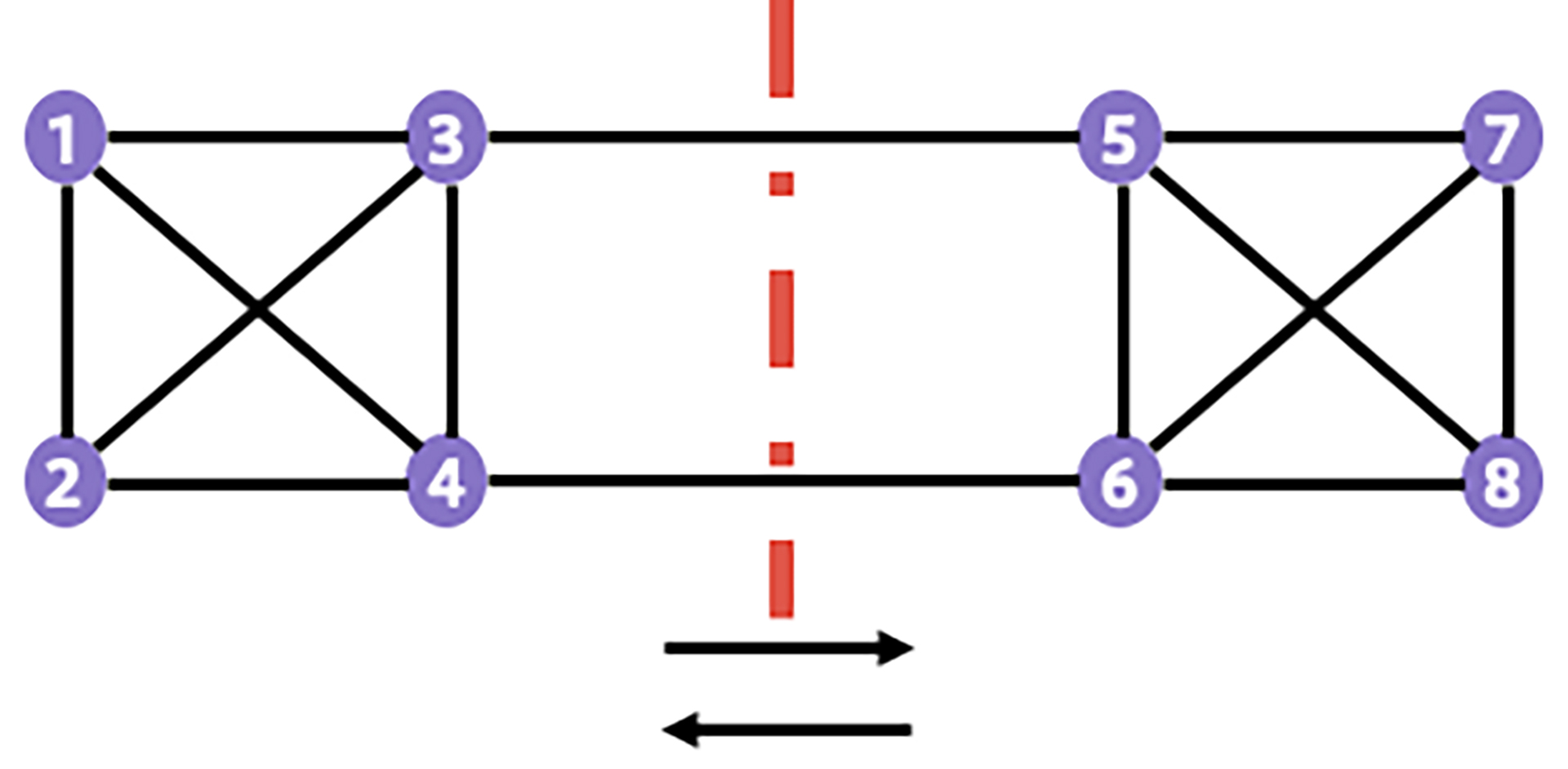
With N nodes there are 2^N possible cuts, but the planar nature of the actual topology simplifies this considerably. Simple cuts, typically straight lines geographically, are more critical for dimensioning than complicated cuts, which are generally covered by a combination of simple ones.
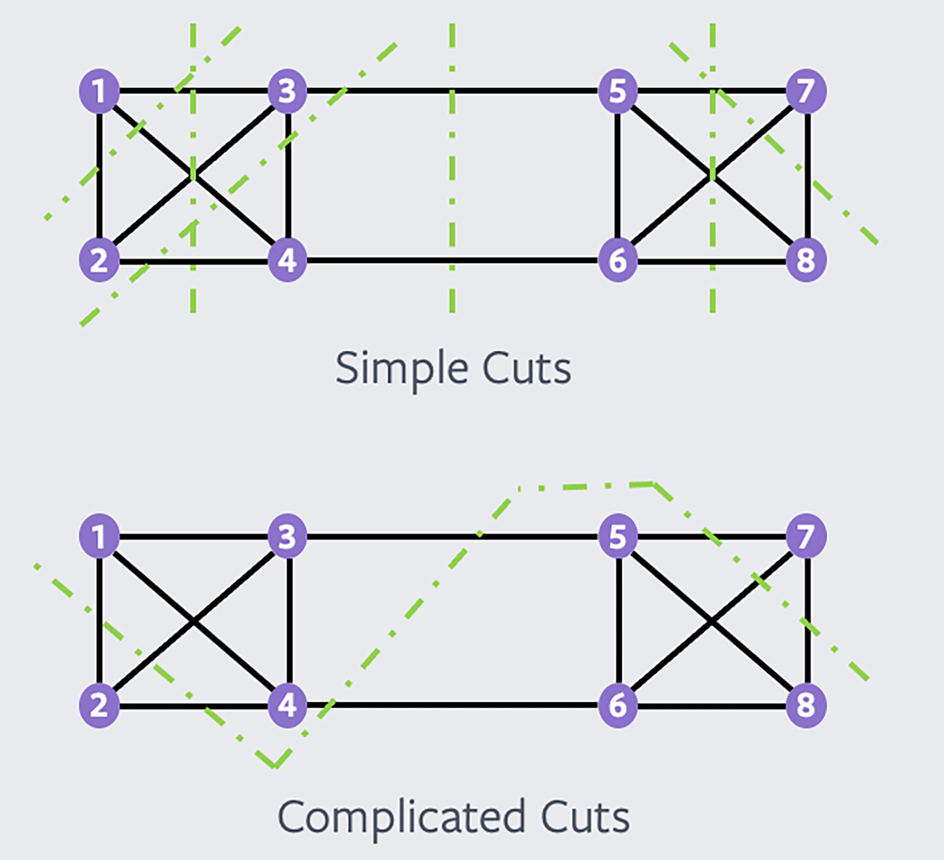
Focusing on simple cuts narrows the set of reference demand matrices to the smallest meaningful set. These matrices are then fed to the cost optimization model to produce a network plan that supports every possible traffic matrix satisfying the hose constraints. In simulations, the extra capacity needed to serve the hose-based traffic matrix instead of a pairwise forecast was not significant, but the simplicity gained in planning and operations was substantial.
What the shift buys
Adopting the hose-based planning model cuts forecast complexity by an order of magnitude. Services can now reason about network capacity at the same per-data-center granularity as compute and storage, and operations no longer chase traffic surges between every pair of data centers. Alarms now track aggregate traffic from a data center, which removes a significant number of harmless, surge-related false alarms.