A linear programming approach for optimizing features in ML models

Feature selection as a resource allocation problem

Machine learning models improve as engineers add new features that capture fresh signals. But every feature carries an infrastructure cost — some demand more memory, others need extra CPU or storage. At Facebook’s scale, accepting every proposed feature would quickly exhaust capacity and slow iteration. The challenge is deciding which features earn their keep.

The team approached this by treating the problem as a linear programming exercise. Framing feature selection this way makes it possible to maximize model performance under real infrastructure constraints, test how sensitive that performance is to different limits, and map how services depend on one another.

A simple model with real trade-offs

Consider a simplified version of the problem. Features consume storage (the height of a rectangle) and contribute some measurable gain to the model (a teal square). Capacity is fixed, so not every feature fits.

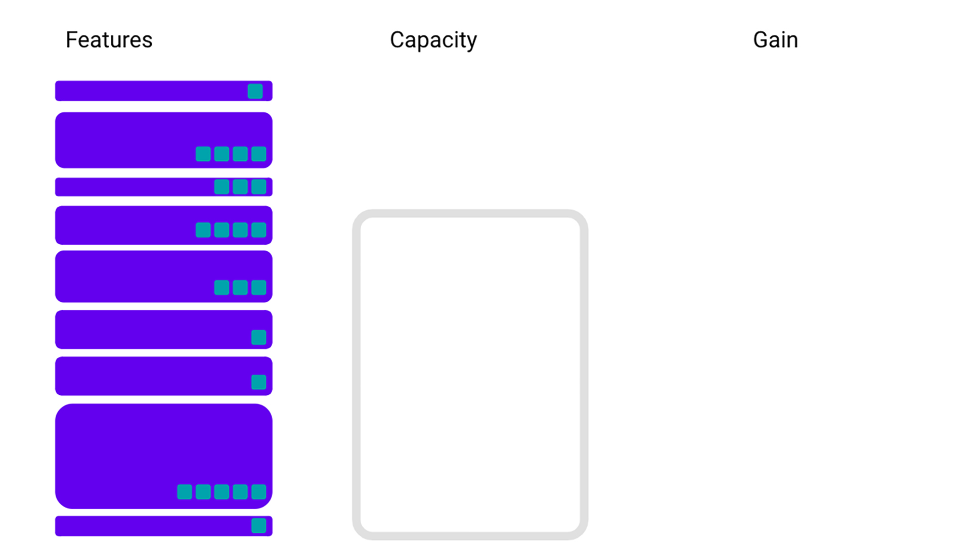
A naive strategy picks the highest-gain features first until space runs out. That can leave capacity idle while smaller, less individually impressive features — which together would outperform the single big one — are excluded.

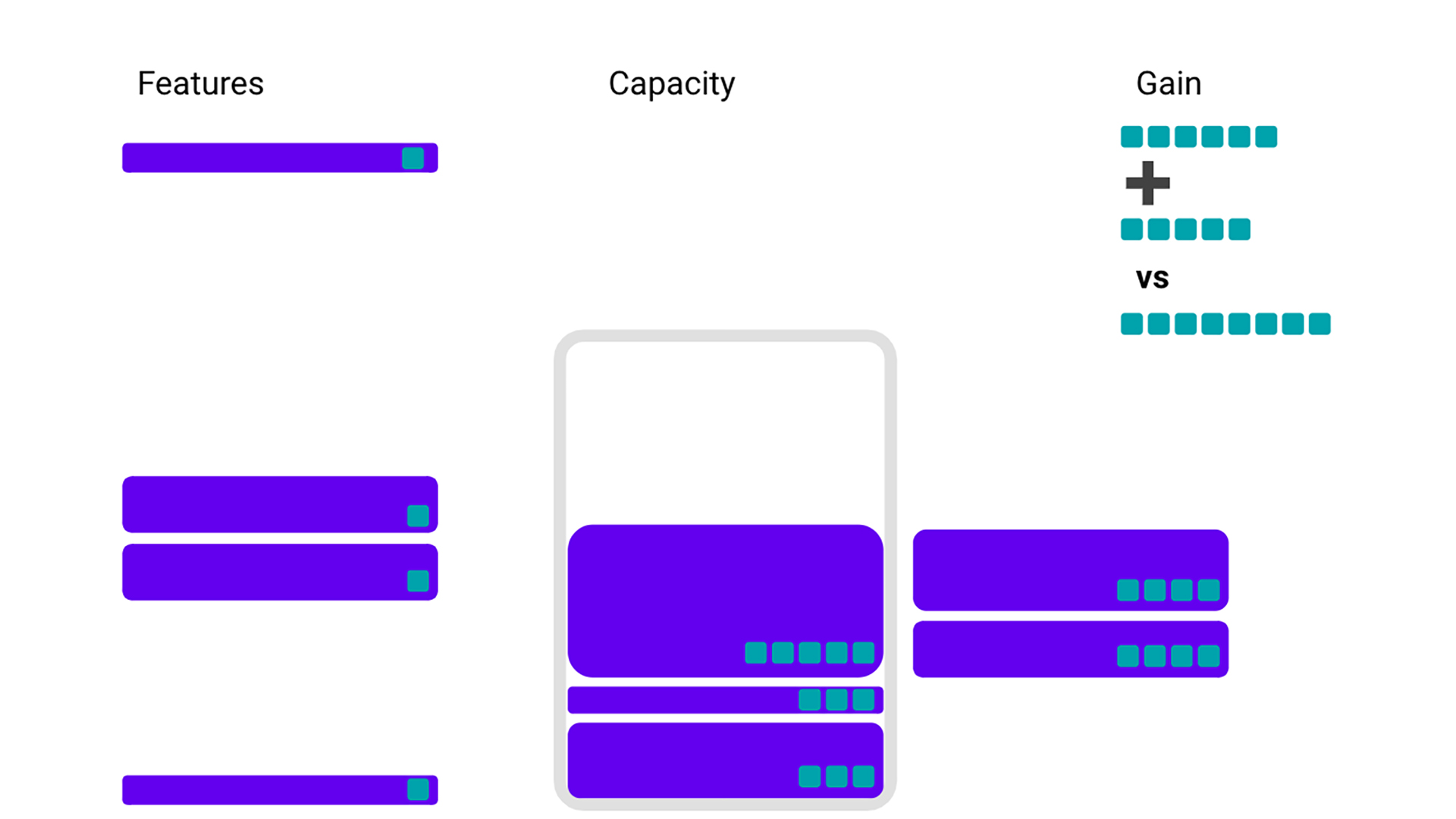
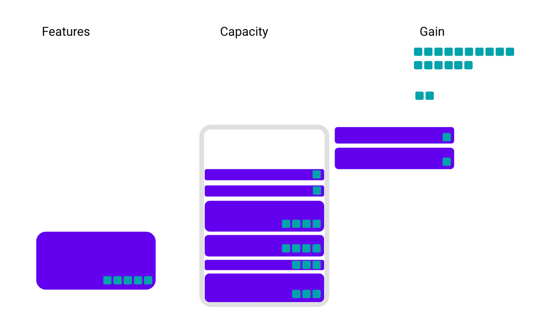
Another approach selects features by gain per unit of storage. That avoids wasted space but risks dropping moderately efficient features that would still fit comfortably.

Real infrastructure complicates this picture. Features rarely consume a single resource. Reintroducing the example, some features draw on both Service A and Service B, so choosing them must respect two separate capacity limits.

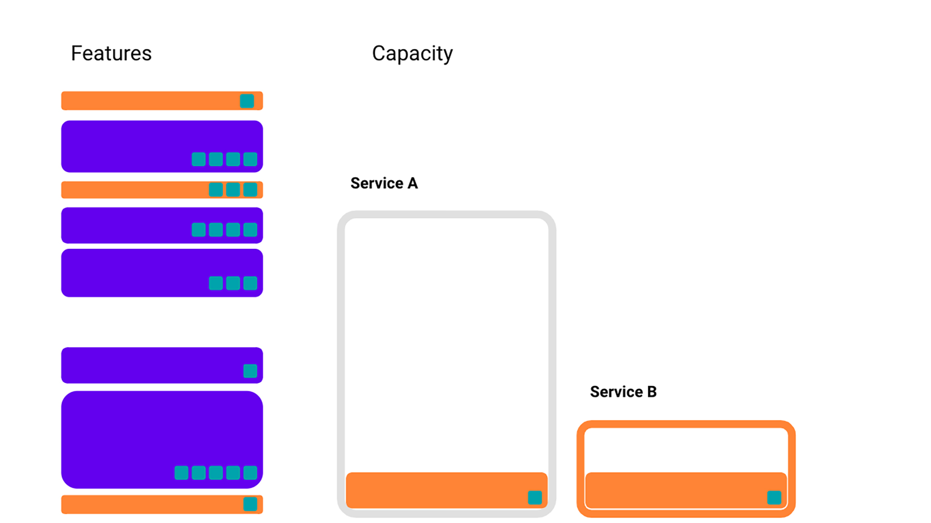
Storage tweaks add another layer. Some features can be compressed to half their original footprint, but compression eats into the feature’s gain and consumes additional Service B capacity — which itself is finite.

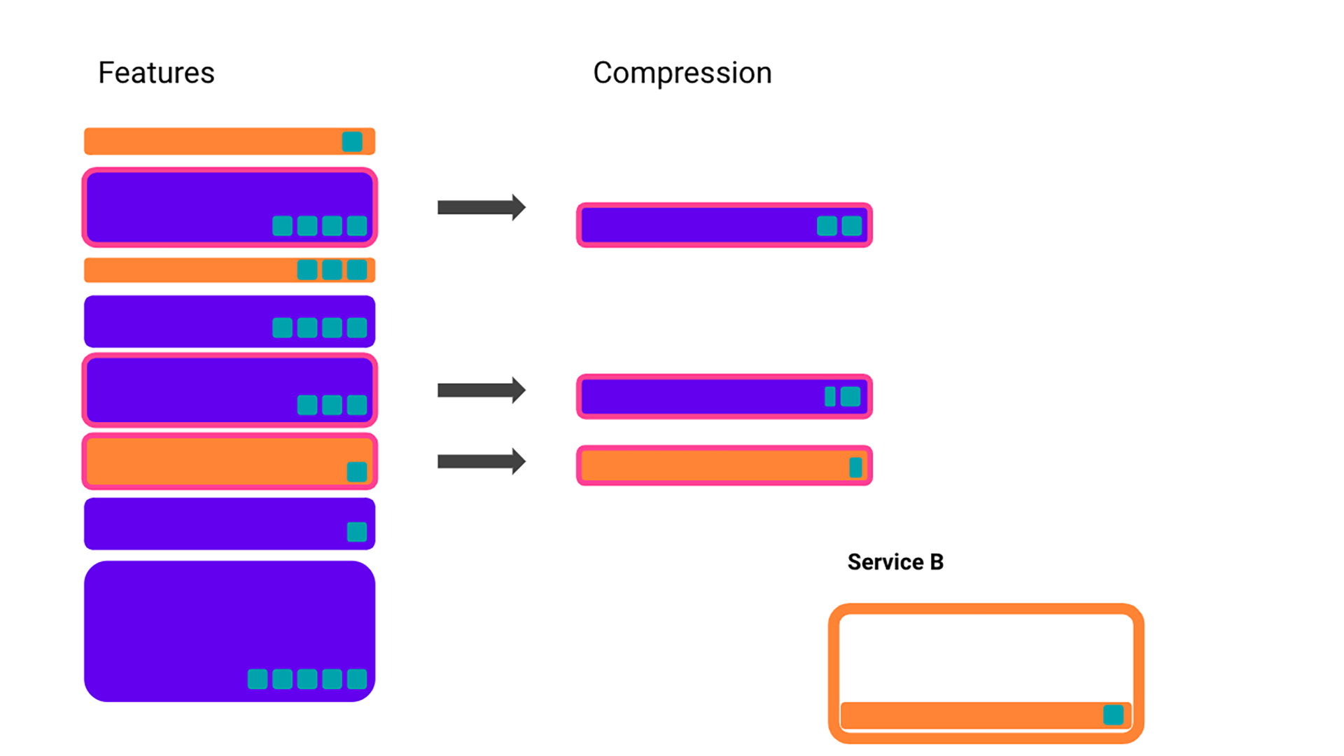
Even this toy model shows how quickly the interacting constraints multiply. In production, capacity is flexible within reason, features are not the only projects competing for space, and the questions we need answered are operational:

• Which features maximize gain given current capacity?
• Does compression pay off — and is it worth engineering time to implement?
• What gain would an extra slice of Service A capacity deliver?
• How do service limits interact — can adding Service B capacity relax the pressure on Service A?

From prose to equations

The model problem can be stated as a small set of conditions:

1. Maximize total gain.
2. Respect the capacity of Service A.
3. Respect the capacity of Service B, which only some features use.
4. Compression is optional but comes with a gain penalty and consumes Service B space.

Those constraints translate directly into linear equations. Let 𝑥 be a binary vector indicating whether a feature is selected, and 𝑔 the vector of feature gains. Subscripts 𝑓 and 𝑐 denote full versus compressed variants — so 𝑥𝑓 marks selected uncompressed features and 𝑔𝑐 holds compressed feature gains. The objective is:

Three constraint groups complete the specification:

1. A feature may be selected compressed, selected uncompressed, or not at all — never both variants simultaneously.

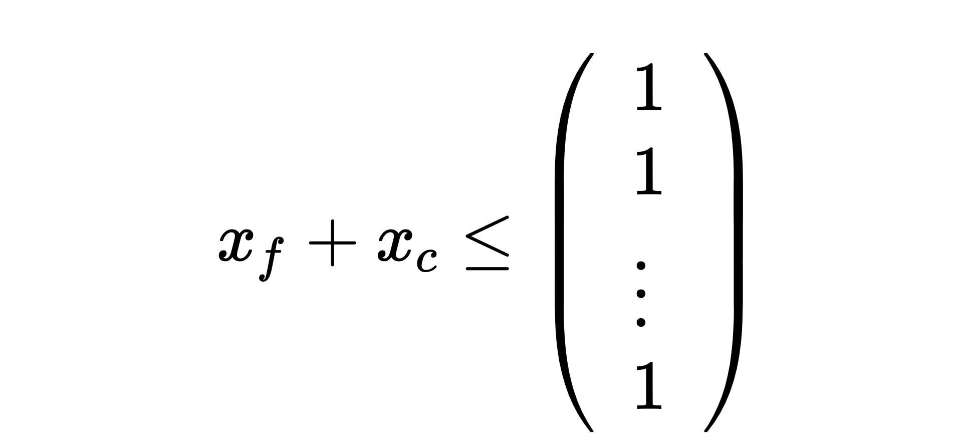
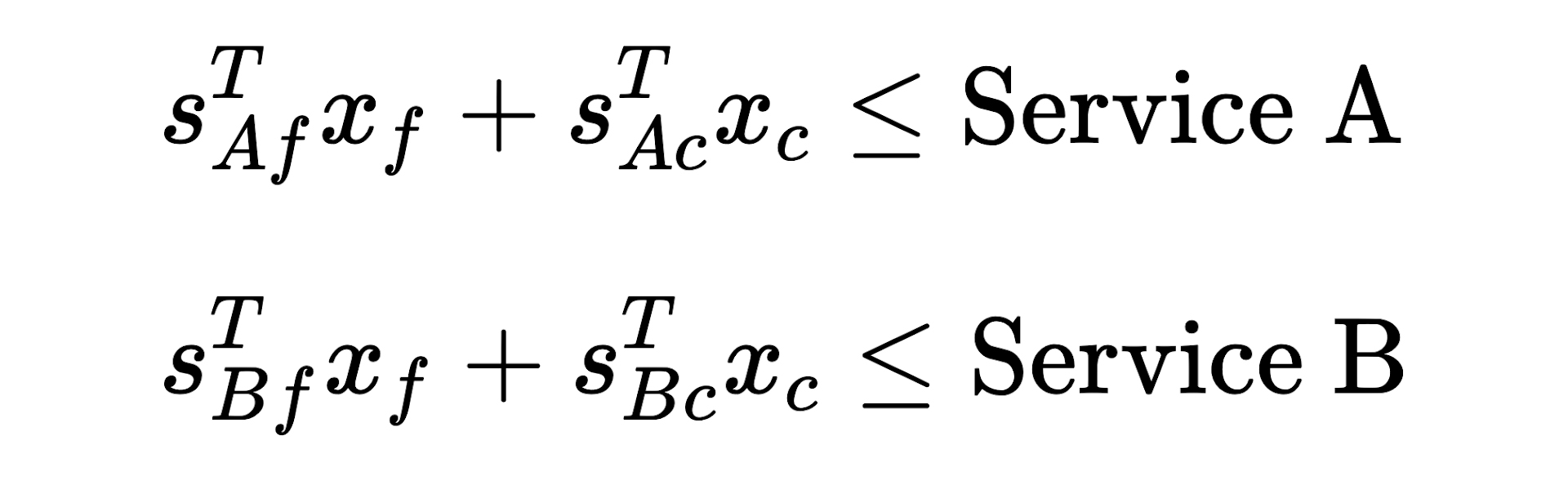
2. Let 𝑠 be the storage cost, subscripted by service (𝐴, 𝐵) and variant (𝑓, 𝑐). Both services are capacity-bound.

3. Compression itself requires some Service B capacity — modeled as a set of features that must be selected.

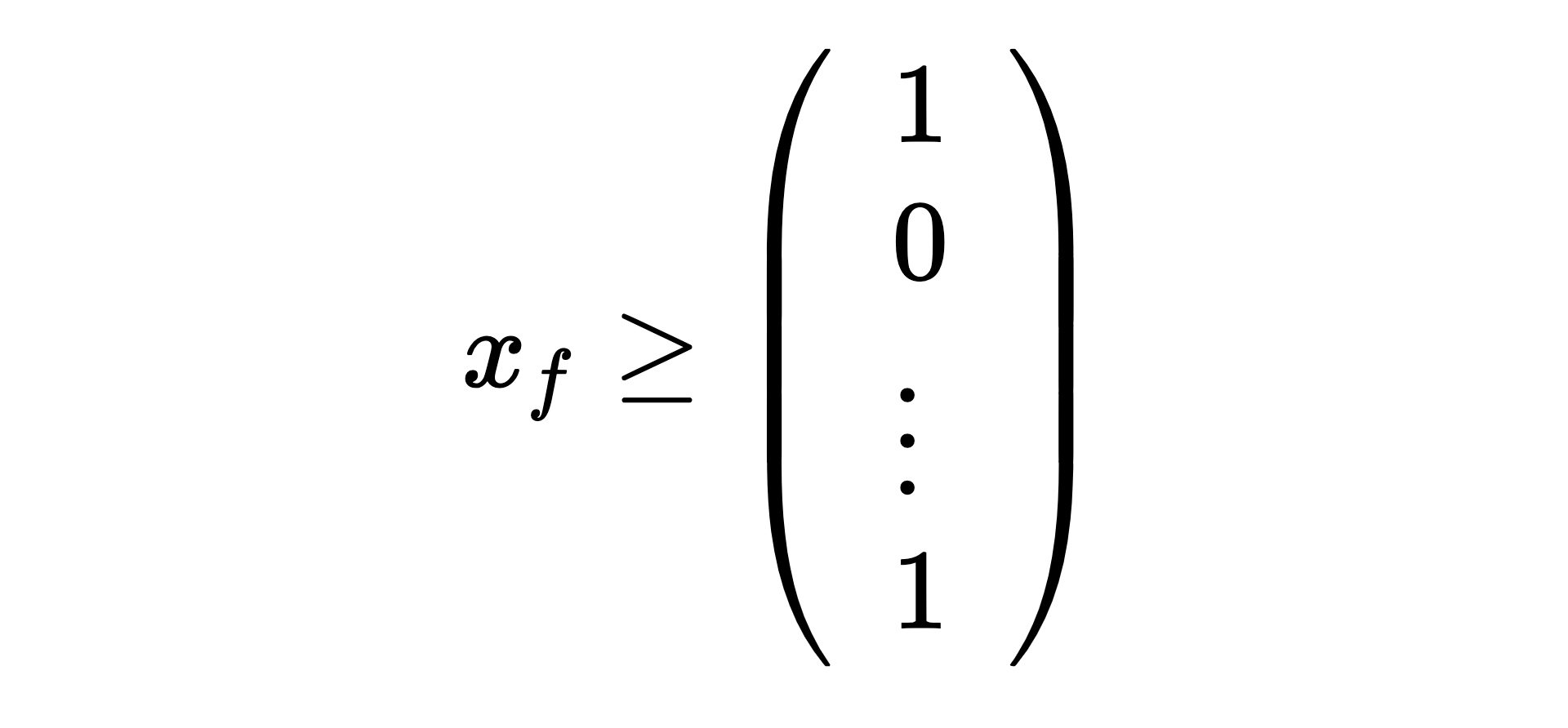
The whole problem reduces to a few equations solvable with standard linear programming tools. For automation, the team implemented it in Python using NumPy and CVXPY.

import cvxpy as cp
import numpy as np
import pandas as pd
 
# Assuming data is a Pandas DataFrame that contains relevant feature data
data = pd.DataFrame(...)
# These variables contain the maximum capacity of various services
service_a = ...
service_b = ...
 
selected_full_features = cp.Variable(data.shape[0], boolean=True)
selected_compressed_features = cp.Variable(data.shape[0], boolean=True)
 
# Maximize the feature gain
feature_gain = (
   data.uncompressed_feature_gain.to_numpy() @ selected_full_features
   + data.compressed_feature_gain.to_numpy() @ selected_compressed_features
)
 
constraints = [
   # 1. We should not select the compressed and uncompressed version
   #    of the same feature
   selected_full_features + selected_compressed_features <= np.ones(data.shape[0]),
   # 2. Features are restricted by the maximum capacity of the services
   data.full_storage_cost.to_numpy() @ selected_full_features
   + data.compressed_storage_cost.to_numpy() @ selected_full_features
   <= service_a,
   data.full_memory_cost.to_numpy() @ selected_full_features
   + data.compressed_memory_cost.to_numpy() @ selected_compressed_features
   <= service_b,
   # 3. Some features must be selected to enable compression
   selected_full_features >= data.special_features.to_numpy(),
]

What the framework answers

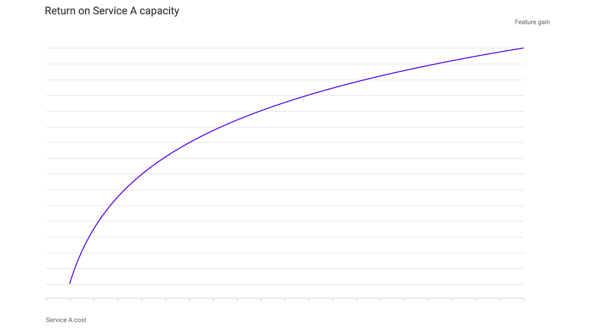
Once the problem is framed this way, hypothetical questions become runs of the optimizer. Vary Service A’s capacity, resolve, and plot the resulting gain. The curve directly quantifies the return from each incremental unit of capacity — a concrete signal for where to invest next, whether in feature memory, compute, or storage.

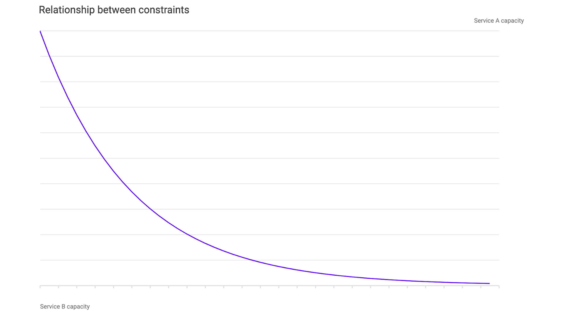
The same approach exposes relationships between services. Holding gain constant and varying the capacities of Services A and B shows, for example, that more Service B capacity reduces how much Service A is needed to hit the same target. That insight matters when one service is under strain and another has headroom.

From manual approval to automated decisions

Feature approval used to be a manual process. Teams spent time estimating how many features infrastructure could support and calculating the payoff of expanding any given service. At Facebook’s scale, with multiple models in continuous development, that process did not scale. Encoding the system as linear equations turns a tangle of interdependent services into relationships that are easy to express, compute, and communicate — and it makes both feature deployment and infrastructure investment decisions far more tractable.