
Why cubic-bezier() matters
Complex CSS animations usually arrive as expansive @keyframes blocks stuffed with declarations. Two techniques reduce that weight while keeping everything in vanilla CSS: running multiple animations at once, and choosing timing functions deliberately. The first is familiar; the second is rarer, and the reason is understandable — chaining animations by comma is easier than internalizing what each timing function does. The most flexible of them is cubic-bezier(), which gives full control over the easing curve and can produce intricate motion with only two keyframes.
The canonical demonstration is a ball traced along an infinity (∞) shape. It uses no complex code: just two keyframes and a cubic-bezier() function.
How the function is defined
The specification describes a cubic Bézier easing function as follows:
A cubic Bézier easing function is a type of easing function defined by four real numbers that specify the two control points, P1 and P2, of a cubic Bézier curve whose end points P0 and P3 are fixed at (0, 0) and (1, 1) respectively. The x coordinates of P1 and P2 are restricted to the range [0, 1].

The curve maps time on the x-axis to output on the y-axis, each spanning [0, 1] (or [0% 100%]). For a two-second animation (2s), that correspondence works as follows:
0 (0%) = 0s
1 (100%) = 2s
Animating left from 5px to 20px maps onto the curve like this:
0 (0%) = 5px
1 (100%) = 20px
While x, the time, is always confined to [0 1], y — the output — may exceed that range.
Faking a parabolic curve
Two shapes not directly producible are of particular interest:
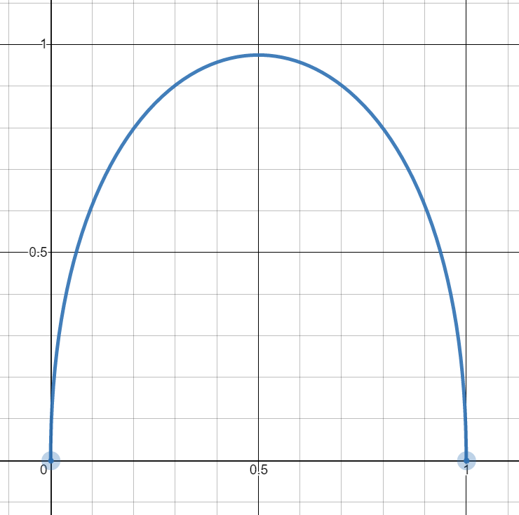
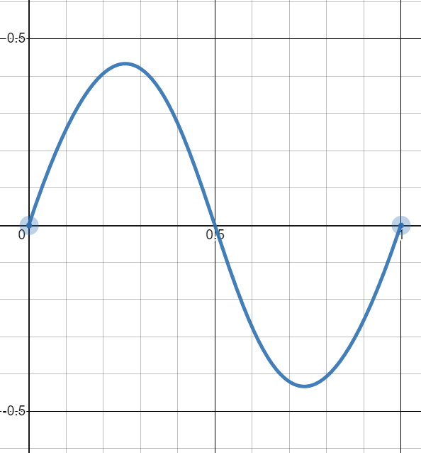
Naively they look impossible, because the definition fixes P0 and P3 at (0,0) and (1,1), so they can never share an axis. The workaround is an approximation built from very large control-point values.
Start with cubic-bezier(0,1.5,1,1.5):
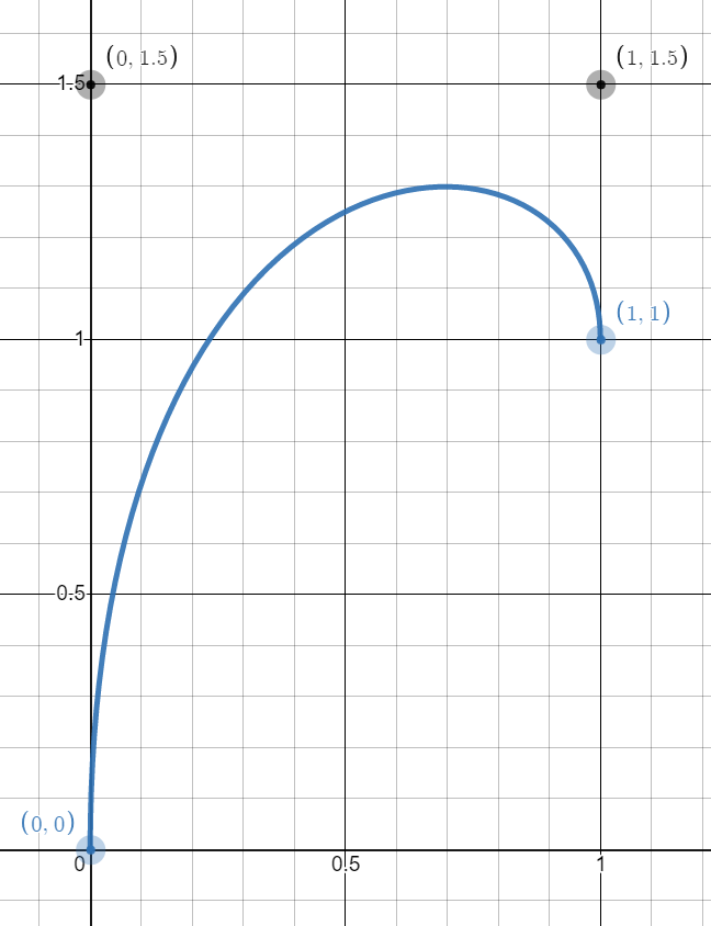
cubic-bezier(0,1.5,1,1.5)The objective is to move (1,1) to (0,1), which isn't technically possible, so we fake it. Since the range is [0 1] (or [0% 100%]), imagine the case where 0% lies very close to 100%. Animating top from 20px (0%) to 20.1px (100%) makes the initial and final states effectively equal.
The element still moves a little, because the y value exceeds 20.1px (100%), but not enough to be perceptible. Raising the curve to cubic-bezier(0,4,1,4):

Still no visible movement, even though top crosses 3 (or 300%). Next try cubic-bezier(0,20,1,20):
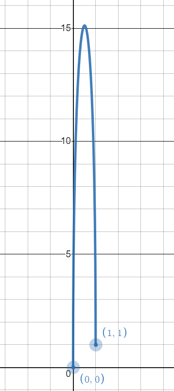
Now motion appears. Each increase effectively drags the point (1,1) "visually" closer to (0,1) when the full curve is viewed zoomed out — that is the trick. Using cubic-bezier(0,V,1,V) with a very large V, combined with initial and final states that are very close together (or nearly equal), simulates the parabolic curve. Applying that curve to a top animation alongside a linear function on left produces the intended motion.
The math behind it
A cubic Bézier is defined by the following formula:
P = (1−t)³P0 + 3(1−t)²tP1 + 3(1−t)t²P2 + t³P3With P0 = (0,0), P1 = (0,V), P2 = (1,V), and P3 = (1,1), the x and y functions become:
X(t) = 3(1−t)t² + t³ = 3t² - 2t³Y(t) = 3(1−t)²tV +3(1−t)t²V + t³ = t³ - 3Vt² + 3Vt
Here V is the large value and t runs over [0 1]. In the top example, Y(t) is the top value and X(t) is time progress; the points (X(t),Y(t)) trace the curve.
The maximum of Y(t) occurs where Y'(t) = 0:
Y'(t) = 3t² - 6Vt + 3VSolving the resulting quadratic gives t = V - sqrt(V² - V). For large V, t approaches 0.5, so Y(0.5) = Max and X(0.5) = 0.5 — the peak lands halfway through the animation, exactly as a parabolic curve requires. Also, Y(0.5) = (1 + 6V)/8, which yields the maximum from V; since V is always large, this simplifies to 6V/8 = 0.75V.
With V = 500, the maximum comes out to 375 (or 37500%), and we get:
- Initial state (
0):top: 200px - Final state (
1):top: 199.5px
The difference between state 0 and 1 is -0.5px — the increment. Multiplying by the maximum: 375*-0.5px = -187.5px, so the element reaches top: 12.5px (200px - 187.5px):
top: 200px (at 0% of the time ) → top: 12.5px (at 50% of the time) → top: 199.5px (at 100% of the time)
Expressed another way:
top: 200px (at 0%) → top: 12.5px (at 50%) → top: 200px (at 100%)Running the logic in reverse: which V makes the element hit top: 0px? The path is 200px → 0px → 199.5px, so -200px of travel is needed and the increment stays -0.5px. The max value is then 200/0.5 = 400, and 0.75V = 400 gives V = 533.33, which brings the element to the top. The figure below sums up the calculation:
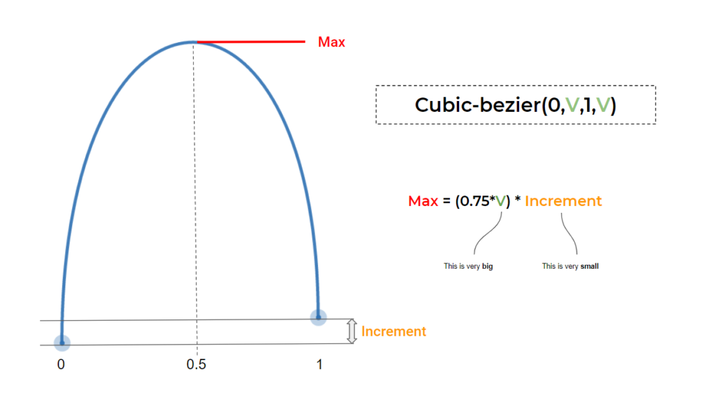
Faking a sinusoidal curve
The sinusoidal shape uses the same trick with a different formula: cubic-bezier(0.5,V,0.5,-V). Increasing the value moves the curve closer to sinusoidal:

With this, a continuous animation becomes a real sinusoidal one.
The math behind it
Following the same formula as before yields:
X(t) = 3/2(1−t)²t + 3/2(1−t)t² + t³ = (3/2)t - (3/2)t² + t³Y(t) = 3(1−t)²tV - 3(1−t)t²V + t³ = (6V + 1)t³ - 9Vt² + 3Vt
This time the minimum and maximum of Y(t) are needed. Setting Y'(t) = 0 gives two solutions:
Y'(t) = 3(6V + 1)t² - 18Vt + 3V = 0…which resolve to:
t' = (3V + sqrt(3V² - V))/(6V + 1)t'' = (3V - sqrt(3V² - V))/(6V + 1)
For large V, t'=0.211 and t"=0.789. Thus Y(0.211) = Max and Y(0.789) = Min, with X(0.211)= 0.26 and X(0.789) = 0.74: the maximum arrives at 26% of the duration and the minimum at 74%. With some rounding for large V, Y(0.211) = 0.289V and Y(0.789) = -0.289V.
A sinusoidal curve should also cross the x-axis (Y(t) = 0) at half the time (X(t) = 0.5). The second derivative confirms it, since Y''(t) = 0:
Y''(t) = 6(6V + 1)t - 18V = 0The solution is 3V/(6V + 1), which for large V is 0.5. So Y(0.5) = 0 and X(0.5) = 0.5, confirming that the curve crosses the (0.5,0) point.
Given:
- Initial state (
0):top: 50% - Final state (
1):top: 49.9% - Increment:
-0.1%
reaching top: 0% requires -50%, so 0.289V*-0.1% = -50%, giving V = 1730.10. The element now touches the top and disappears at the bottom:
top: 50% → top: 0% → top: 50% → top: 100% → top: 50% → and so on ... Here is the calculation summarized:
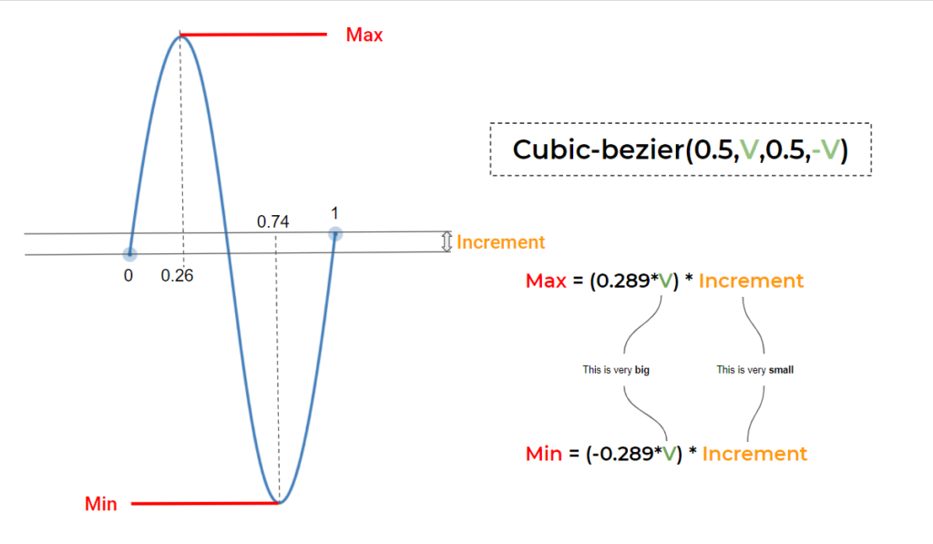
In the four-curves demo, two different animations are in play: one going to 49.9% (increment -0.01%) and one going to 50.1% (increment +0.01%). Flipping the sign of the increment flips the direction of the curve.
Back to the infinity example
The opening ball animation is simply two sinusoidal animations joined together. Combining that approach with multiple animations produces substantial results, and the interactive demo lets you change values and see the effect directly.
A step further: CSS Houdini, via @property, allows a complex transform declaration to be animated — with the caveat that CSS Houdini is currently limited to Chrome and Edge support. The resulting drawings include:

A spirograph animation is also achievable, with and without CSS Houdini. The key takeaways from these examples:
- Each keyframe is defined using only one declaration that contains the increment.
- The position of the element and the animation are independent, so the element can be placed anywhere without adjusting the animation.
- No calculations are required — no piles of angles or pixel values, just a tiny value within the keyframe and a big value within
cubic-bezier(). - The whole animation can be controlled by adjusting the duration value.
Transitions without keyframes
The same technique applies to the CSS transition property, since it follows the same logic for timing functions. That means complex hover effects can be built without any keyframes: a jumping Mario driven by the parabolic curve, plus a shake animation on hover, both from keyframe-free code. The sinusoidal curve handles the bulk of the work, and a CSS Houdini version of the jumping Mario (again, Chrome and Edge only) uses the parabolic curve too; more fancy hover effects are in the same family.
Tools instead of math
Not everyone is math-minded, and plenty of tooling exists for that: Matthew Lein's Ceaser, where curve points are dragged into place; cubic-bezier.com, worth bookmarking; and desmos for playing with cubic-bezier outside CSS, where the formulas can be inspected directly.