Word embeddings, explained
An embedding is a dense vector of floating-point values that represents a word's meaning. The basic intuition: words that are close together in the embedding space should be similar in meaning. Before embeddings, words were typically represented as one-hot vectors—huge, sparse, and semantically meaningless. "Paris" and "France" were as distant as "Paris" and "Armadillo."
Embeddings solved that. By learning a mapping from a vocabulary of words to vectors in a high-dimensional space, models can operate on words in a way that preserves semantic relationships.
The CBOW architecture
The 2013 word2vec paper proposed two architectures: Continuous Bag of Words (CBOW) and Continuous Skip-Gram. CBOW is the simpler of the two and the focus here. The goal: given the context words around a target word, predict the target word itself.
For example, with a window size of four on each side, the model sees something like:
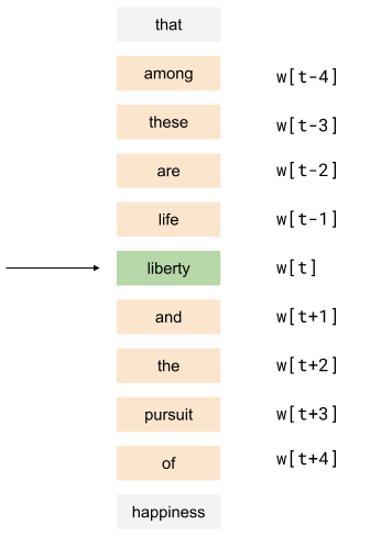
The model must predict the middle word ("liberty") from the eight surrounding context words. This is unsupervised—it learns simply by sliding over arbitrary amounts of text, word by word.
The architecture breaks down into a few steps, with these dimensions:
- B: batch size (processed together for efficiency)
- V: vocabulary size
- D: model depth (the dimension of the learned embeddings)
- W: window size on each side
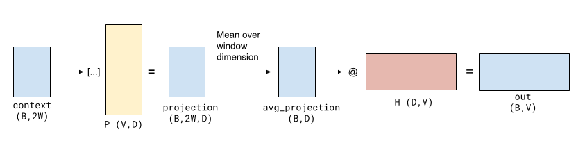
The forward pass works like this:
contextis an array of shape(B, 2W), each element the integer index of a word in the vocabulary.- The context indexes into a projection matrix
P, which holds one embedding per row. This producesprojection, shape(B, 2W, D)—every integer index is replaced by its dense embedding vector. - The embeddings within each window are averaged, producing a
(B, D)tensor of context-mean embeddings. - A hidden layer matrix
Hmaps this back to vocabulary space—a sparse prediction of the middle word's one-hot index.
During training, the output is compared against the true one-hot target word, and the gradient is backpropagated to update P and H.
A compact JAX implementation
The whole model in JAX is remarkably small:
@jax.jit
def word2vec_forward(params, context):
    """Forward pass of the word2Vec model.

    context is a (batch_size, 2*window_size) array of word IDs.

    V is the vocabulary size, D is the embedding dimension.
    params["projection"] is a (V, D) matrix of word embeddings.
    params["hidden"] is a (D, V) matrix of weights for the hidden layer.
    """
    # Indexing into (V, D) matrix with a batch of IDs. The output shape
    # is (batch_size, 2*window_size, D).
    projection = params["projection"][context]

    # Compute average across the context word. The output shape is
    # (batch_size, D).
    avg_projection = jnp.mean(projection, axis=1)

    # (batch_size, D) @ (D, V) -> (batch_size, V)
    hidden = jnp.dot(avg_projection, params["hidden"])
    return hidden

@jax.jit
def word2vec_loss(params, target, context):
    """Compute the loss of the word2Vec model."""
    logits = word2vec_forward(params, context)  # (batch_size, V)

    target_onehot = jax.nn.one_hot(target, logits.shape[1])  # (batch_size, V)
    loss = optax.losses.softmax_cross_entropy(logits, target_onehot).mean()
    return loss
Training details
Training uses the same dataset as the original word2vec code—a 100 MB text file of lowercased, punctuation-free text from http://mattmahoney.net/dc/text8.zip. Because it's already clean, preprocessing is minimal—except for subsampling: common words like "and" and "is" appear so frequently that they need to be randomly discarded for the model to learn meaningful representations.
def subsample(words, threshold=1e-4):
    """Subsample frequent words, return a new list of words.

    Follows the subsampling procedure described in the paper "Distributed
    Representations of Words and Phrases and their Compositionality" by
    Mikolov et al. (2013).
    """
    word_counts = Counter(words)
    total_count = len(words)
    freqs = {word: count / total_count for word, count in word_counts.items()}

    # Common words (freq(word) > threshold) are kept with a computed
    # probability, while rare words are always kept.
    p_keep = {
        word: math.sqrt(threshold / freqs[word]) if freqs[word] > threshold else 1
        for word in word_counts
    }
    return [word for word in words if random.random() < p_keep[word]]
The next step is fixing a vocabulary size:
def make_vocabulary(words, top_k=20000):
    """Creates a vocabulary from a list of words.

    Keeps the top_k most common words and assigns an index to each word. The
    index 0 is reserved for the "<unk>" token.
    """
    word_counts = Counter(words)
    vocab = {"<unk>": 0}
    for word, _ in word_counts.most_common(top_k - 1):
        vocab[word] = len(vocab)
    return vocab
The preprocessed subsampled words and vocabulary are stored in a pickle file. The training loop then trains from random initialization, using hyper-parameters chosen to match the original word2vec code:
def train(train_data, vocab):
    V = len(vocab)
    D = 200
    LEARNING_RATE = 1e-3
    WINDOW_SIZE = 8
    BATCH_SIZE = 1024
    EPOCHS = 25

    initializer = jax.nn.initializers.glorot_uniform()
    params = {
        "projection": initializer(jax.random.PRNGKey(501337), (V, D)),
        "hidden": initializer(jax.random.PRNGKey(501337), (D, V)),
    }

    optimizer = optax.adam(LEARNING_RATE)
    opt_state = optimizer.init(params)

    print("Approximate number of batches:", len(train_data) // BATCH_SIZE)

    for epoch in range(EPOCHS):
        print(f"=== Epoch {epoch + 1}")
        epoch_loss = []
        for n, (target_batch, context_batch) in enumerate(
            generate_train_vectors(
                train_data, vocab, window_size=WINDOW_SIZE, batch_size=BATCH_SIZE
            )
        ):
            # Shuffle the batch.
            indices = np.random.permutation(len(target_batch))
            target_batch = target_batch[indices]
            context_batch = context_batch[indices]

            # Compute the loss and gradients; optimize.
            loss, grads = jax.value_and_grad(word2vec_loss)(
                params, target_batch, context_batch
            )
            updates, opt_state = optimizer.update(grads, opt_state)
            params = optax.apply_updates(params, updates)

            epoch_loss.append(loss)
            if n > 0 and n % 1000 == 0:
                print(f"Batch {n}")

        print(f"Epoch loss: {np.mean(epoch_loss):.2f}")
        checkpoint_filename = f"checkpoint-{epoch:03}.pickle"
        print("Saving checkpoint to", checkpoint_filename)
        with open(checkpoint_filename, "wb") as file:
            pickle.dump(params, file)
The generate_train_vectors function is straightforward bookkeeping, available in the full code. Training 25 epochs on a modest GPU takes around 20–30 minutes.
Extracting embeddings and similar words
After training, the P matrix is the embedding table: each row maps a word to its embedding. With it, word-similarity demos are straightforward. Examples:
$ uv run similar-words.py -word paris \
      -checkpoint checkpoint.pickle \
      -traindata train-data.pickle
Words similar to 'paris':
paris           1.00
france          0.50
french          0.49
la              0.42
le              0.41
henri           0.40
toulouse        0.38
brussels        0.38
petit           0.38
les             0.38
$ uv run similar-words.py -analogy berlin,germany,tokyo \
      -checkpoint checkpoint.pickle \
      -traindata train-data.pickle
Analogies for 'berlin is to germany as tokyo is to ?':
tokyo           0.70
japan           0.45
japanese        0.44
osaka           0.40
china           0.36
germany         0.35
singapore       0.32
han             0.31
gu              0.31
kyushu          0.31
The underlying principle: words with similar meanings appear near similar context words. The model learns to internalize this, and can even capture analogies:
$ uv run similar-words.py -sims soccer,basketball,chess,cat,bomb \
      -checkpoint checkpoint.pickle \
      -traindata train-data.pickle
Similarities for 'soccer' with context words ['basketball', 'chess', 'cat', 'bomb']:
basketball      0.40
chess           0.22
cat             0.14
bomb            0.13
Optimizations left out
The word2vec authors later documented several optimizations in a follow-up paper—most aimed at avoiding the final expensive multiplication by H. These can substantially improve quality by allowing larger D and bigger training corpora. They're omitted here for clarity, and because word2vec itself has largely been superseded by modern transformer-based embedding training.
Running the original C code
The original word2vec project page on Google Code still has useful documentation, but its Subversion instructions are dead. A GitHub mirror lives at https://github.com/tmikolov/word2vec. The code compiles and runs with a simple make, and the included shell scripts handle data download and training. It's CPU-based and slow, but reproduces the similarity results without trouble.
How modern LLMs handle embeddings
Word2vec trained a standalone embedding matrix for use by other models. That's mostly history now. In GPT-style transformers, the embedding matrix appears as the model's first layer—the same role as P in CBOW—but it's trained jointly with the rest of the network. This makes sense for two reasons:
- LLMs consume enormous amounts of text; separately pre-training embeddings on that data would be wasteful.
- Embeddings co-trained with the model better match its tokenizer, depth, and task.
Two differences stand out between word2vec-style embeddings and modern ones:
- Tokens, not words. Modern models embed sub-word tokens, a key shift in how language is represented for machines.
- Much larger depth. GPT-3 uses
D=12288; newer models go even higher. Larger embeddings capture finer semantic nuances, but require substantially more data to train.
Full runnable code and instructions are available in the repository README.