Projections and Projection Matrices - Eli Bendersky's website

Projection as a Geometric Operation

A projection is best understood visually: for a vector b, its projection onto a line or a plane is the closest point in that subspace to b — equivalently, the "shadow" of b cast by a light source perpendicular to the target subspace.

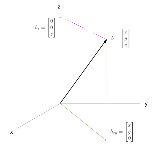
Projections onto coordinate axes are simple: projecting a 3D vector onto the z axis yields a vector with just the z-component retained. The same logic extends to arbitrary lines rather than just coordinate axes.

Projecting onto a Line

In vector space, a line through the origin is the set of all scalar multiples of a fixed vector a. For a target vector b, we seek the projection vector p that is a scalar multiple of a — the closest such vector to b.

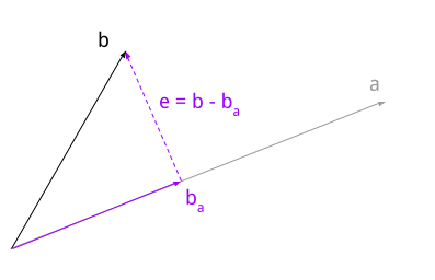
The key geometric constraint is that the error vector b-p is orthogonal to a. Since p = ca for some scalar c, orthogonality gives:

a·(b - ca) = 0

Expanding using the distributive property of the dot product:

a·b = c(a·a)

Here, a·a is the squared magnitude of a. Thus, whether a is a unit vector is immaterial — the formula inherently normalizes it.

From Scalar to Projection Matrix

Switching to matrix notation (vectors as columns), the dot product becomes a matrix product between a row and a column vector. Defining P as the projection matrix for vector a, we have:

P = a(aTa)-1aT = aaT/(aTa)

For a 3D vector a, aa^T is a 3×3 matrix and the denominator is a scalar. The projection of any vector b onto the line spanned by a is then simply Pb.

Worked Example: Line Projection

Returning to the original z-axis case: the unit vector along z is (0,0,1). Its projection matrix becomes:

P = [[0,0,0],[0,0,0],[0,0,1]]

Multiplying an arbitrary b = (bx, by, bz) by P yields (0, 0, bz), as expected.

For a less trivial direction, take the line spanned by:

a = (2, 1, 2)

Its projection matrix calculated via the formula above is:

P = 1/9 * [[4, 2, 4], [2, 1, 2], [4, 2, 4]]

For a target vector b of (1, 1, 1), projecting:

b_proj = P*b = (10/9, 5/9, 10/9)

Verifying orthogonality: the error vector is (-1/9, 4/9, -1/9), and its dot product with a is zero — confirming the projection is correct.

General Projection onto Subspaces

The line projection is a special case of projecting onto a subspace. For n linearly independent vectors spanning an m-dimensional space, we arrange them as columns of matrix A. The projection of vector b onto this span is some linear combination of the columns — expressed as Ac for a coefficient vector c.

The error vector b - Ac must be orthogonal to every column of A, which gives the system:

AT(b - Ac) = 0

Rearranging and solving:

c = (ATA)-1ATb

The projection matrix then becomes:

P = A(ATA)-1AT

This holds for a line as well: when A has a single column, the formula reduces to the case derived earlier. Linearly independent columns guarantee that A^TA is invertible, making the expression valid.

Example: Projection onto a Plane

Consider the projection onto the xy-plane from the introductory diagram, spanned by the standard basis vectors (1,0,0) and (0,1,0). Stacking them:

A = [[1,0],[0,1],[0,0]]

Here, A^TA is the 2×2 identity, so its inverse is itself. The projection matrix is therefore:

P = [[1,0,0],[0,1,0],[0,0,0]]

As expected, multiplying any vector by P simply zeroes out its z-component. For a general plane spanned by non-orthogonal independent vectors, the same procedure yields a valid projection matrix.

Two Structural Properties

Symmetry

Projection matrices are symmetric: PT = P. Using the transpose rule for products and the fact that the inverse of a symmetric matrix is symmetric, transposing the definition yields:

PT = (A(A^TA)^-1A^T)^T = A((A^TA)^T)^-1A^T = P

Idempotence

Projection matrices are also idempotent: applying the projection twice gives the same result as once. Algebraically, P2 = P, since projecting b to Pb lands in the subspace, and projecting — best approximation at Pb — yields Pb again.

Complementary Orthogonal Subspaces

Working with mutually orthogonal vectors yields a particularly clean case. Consider vector a₁ and its projection matrix P₁. For an orthogonal vector a₂, its projection matrix P₂ is constructed analogously.

Because P₁ + P₂ itself satisfies the symmetry and idempotence properties, the sum is itself a valid projection matrix.

Generalizing: if the vectors a₁ through a_k are mutually orthogonal — forming an orthogonal basis — then the sum of their individual projection matrices corresponds to projecting onto the entire spanned subspace. When those vectors span the whole m-dimensional space, this sum is simply the identity matrix:

Ib = (P1 + P2 + ... + Pk)b

This identity merely restates b in an alternative orthogonal basis — a fact that ties the projection-matrix framework back to basic coordinate transformations.