
Why Aggregate Metrics Mislead
Sampled success metrics, such as conversion rate or checkout completion, are routinely summarized as a single aggregate number. That summary is treated as if it were an exact ground-truth measurement. In reality, the number is a statistic computed from a finite sample, and sampling noise can make two processes that are truly identical appear different — or hide a genuine difference behind random variation.
The core problem is that a binary success event (did the user convert, or not) has inherent variance. Run a checkout flow with a 2% conversion rate twice, and you will rarely observe exactly 2% in both runs. Each run yields a slightly different fraction because users are effectively draws from a distribution. The observed rate is an estimate of the true rate, and the width of the estimation error depends on the sample size.
When decision makers compare two variants — say, a control and a treatment group — they are often comparing two noisy estimates against each other. A gap that appears in the data may be entirely explainable by random fluctuation. This becomes especially dangerous when the sample is small, or when the success event is rare, because both conditions inflate the variance of the estimate.
A Visual Sanity Check
A quick way to develop intuition for sampling noise is to simulate draws from a known distribution. If the true conversion rate is p = 0.02 and you simulate n = 300 trials, the observed rate will jump around. Repeating that simulation many times produces a distribution of observed rates — none of which exactly equals the 0.02 used to generate the data. This is not a bug in the experiment; it is the mathematical consequence of sampling.
This exercise reveals two important facts. First, small samples yield wide distributions of observed outcomes. Second, rare events (low p) need dramatically larger samples to achieve the same relative precision. Both facts argue against making decisions from a single point estimate.
Defining a Decision Rule
Instead of eyeballing the aggregate difference, a defensible position requires a decision rule that acknowledges uncertainty. A standard approach is to construct a confidence interval for the difference between two rates. If that interval does not contain zero, you have statistical evidence of a difference. If it contains zero, the data is consistent with no difference.
That logic suffers the usual pitfalls of null-hypothesis testing: significance depends on sample size, and "not significant" is not the same as "equal." What is needed in practice is a decision threshold that carries a business meaning — for example, "we will ship the treatment if we are confident it improves the rate by at least X, and we are willing to accept that we will be wrong Y% of the time."
Bayesian Decision Making with Simulations
A Bayesian approach fits naturally here. Rather than computing a point estimate and a confidence interval, treat the unknown true conversion rates as random variables with a posterior distribution. From that posterior you can directly query the quantities you care about: the probability the treatment beats control, the probability the improvement exceeds a threshold, or the expected loss of shipping a bad variant.
A Monte Carlo simulation is the workhorse for computing these quantities. Draw many joint samples of the two rates from their posterior. For each draw, compute the difference diff = p_treatment - p_control. After tens of thousands of draws, you have a full empirical distribution over the difference. Summarize it with percentiles: the 2.5th to 97.5th percentile gives you a credible interval, and the fraction of draws where diff > 0 gives you the posterior probability of improvement.
The advantage of this framing is that the decision rule is explicit. You can say, "We will ship the treatment if at least 95% of the posterior mass lies above zero," or "…above an effect size we care about." This separates the question of statistical evidence from the question of business impact.
Posterior Distributions for Rates
For binary outcomes with a prior Beta(1, 1) (uniform), the posterior on p given k successes in n trials is Beta(1 + k, 1 + n - k). In simulation you do not solve this algebraically; you sample from each beta distribution and compare. Updating the prior over multiple recorded drivers — time-of-day, device type, cohort — can be done hierarchically by placing these posters as priors and pooling or learning from data in a drill-down, while formally modeling the interdependence to avoid overstating confidence when slicing groups.
This drill-down is powerful but must be disciplined. Post-hoc subgroup analysis of a noisy metric is a natural factory for false positives that masquerade as insight. Without accounting for multiplicity — the fact that looking at many slices increases the chance one of them shows a spurious effect — you will regularly find "effects" that vanish on the next replication.
Framework Implementation
Use a simulation loop as an alternative to closed-form bandit calculations or legacy t-tests. At every decision point — daily recap, campaign-end report, feature gate — run a finite number of trial samples from the posterior of each variant in play, save the comparison statistics, and feed the decisions into the next step of the optimization. Over a feature experiment, the typical run would compare one control against several variants at once, using nested rbeta calls as the simulation.
An advantage of working with a Monte Carlo engine is that the quantity you aggregate is the quantity you evaluate later. As new events come in, you add them to the observed successes and trials per variant and resample the relevant decision criteria, keeping the posterior consistent. In production usage at scale, tens of thousands of draws on ≤ ten active variants per experiment resolves within a second on standard web infrastructure — fast enough to serve through the API at request time.
The heart of correct inference lies in specifying the event construction: the funnel criterion of "success" has to persist through the entire lifecycle. If a conversion is treated as a single collapsed flag at week-end, then a drill-down that reassigns events to a subgroup cannot fix the funnel criteria, skewing the posterior when you segment by something like device or traffic source while counting pre-cancellation events.
When the Effect Isn't Real
An illustrative case: a control metric sits at 0.029% and the treatment at 0.031%. On thousands of events the aggregate wins. But on drill-down by a side attribute that the variant changed, the treatment rate spikes in the slice while the control loses confidence because the drill triggers fewer sampled events and the mean estimate carries more uncertainty. Instead of trusting a sudden slice, inspect the marginal quality and result against the relevant deltas in the controlled event space. If neither carries a statistically meaningful difference, the slice is noise — a visualization of variance, not signal.
This is why preserving the pre-registered primary metric for any go/no-go decision is wise. Drill-downs generate hypotheses for your next experiment, not for the one you just ran.
Key Takeaways
- Representing a metric by a point estimate invites sampling noise to masquerade as a discovery of "change." The surprising
τ— absolute difference over baseline — remains a recommendation when seen after simulation if the delta is smaller than its uncertainty over the observed window. - With core parameters flattened into a few stochastic fields, a simulation naturally forecasts the true precision level across flags, period, success thresholds, and dilution factors — no separate planning model required.
- Monte Carlo is a decision-friendly layer essential to any mid- to high-funnel success criterion. It supports extracting a quantitative product discussion while lowering the surface for future error terms.
Monte Carlo Simulations: Separating Signal from Noise in Sampled Success Metrics

Most success metrics can be measured directly. At Shopify, for instance, we can calculate Gross Merchandise Volume (GMV) to the penny because every order lives in our databases. But some metrics aren't so easy to capture. When the data needed to evaluate impact is unavailable, too expensive, or simply impractical to collect in full, you fall back on a sampled success metric.
Sampled metrics bring their own problem. In a one-off experiment, you can compute the sample size required for a target confidence interval. But success metrics are usually tracked over time, and each data point matters only in the context of the trend. Confidence accumulates. So how do you extract a real signal from the sampling noise that surrounds each monthly observation? A Monte Carlo simulation is a practical way to answer that.
The technique lets you generate many random inputs based on real-world assumptions, push them through a function that approximates your situation, and inspect the spread of outputs. For a sampled success metric, you can use it to explore the tradeoff between sample size and your ability to spot changes in the underlying population metric. It also gives you a concrete way to brief non-technical stakeholders: instead of abstract statistical language, you can show the percentage of certainty a given sample size yields against the cost of gathering more data.
Defining the Simulation Metrics
To illustrate the method, we'll look at the Shopify App Store. With over 8,000 apps and more than 200 minimum requirements covering security, functionality, and ease of use, the store maintains quality through manual and automated review processes. The question leadership cares about is straightforward: are these processes improving app quality? Quantitatively, we can phrase it as the shop issue rate — the number of requirement violations merchants experience with the average installed app. Since auditing every app daily isn't feasible, we sample a random set monthly to estimate this rate and track it over time.
Before simulating, we need metrics that describe the behavior of our sampled success metric itself. We define a bespoke metric called 1 month decrease observed (1mDO): given a hypothesized monthly decrease in the underlying population issue rate, in what percentage of months does our sampled metric actually go down? We can extend this to two consecutive months (2mDO) or a full quarter (1qDO). We also track mean absolute percentage error (MAPE) to quantify how far the sampled shop issue rate strays from the true population value each month.
Choosing a Distribution
The simulation draws inputs from a defined distribution. For app issues, the Poisson distribution is a good fit: the count of issues across many independent requirement checks behaves like the sum of Bernoulli trials. With a Poisson distribution, a single parameter λ specifies both the mean and the variance. If your metric follows a different pattern — a normal distribution, for instance — you'll need to specify the mean and variance separately. If you don't have sample data to estimate these parameters, the simulation allows you to test outcomes across different assumptions.
Simulating Realistic Time Series
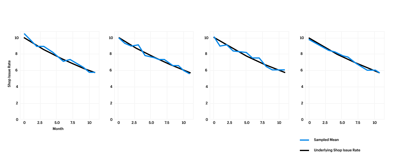
We start with a building-block function that generates a sampled time series under fixed assumptions. For this example, assume the population mean is 10 issues per install (the λ parameter) and that our review processes reduce the issue rate by 5 percent per month. The function draws n=audits_per_period apps each month for m=periods months from that shrinking Poisson distribution. The chart below shows how the sampled shop issue rate fluctuates around the true decreasing trend.

From one simulated series we can compute MAPE and 1mDO. In our first run, MAPE came in at 4.3 percent, meaning the sampled metric typically missed the population mean by that margin. 1mDO was 72 percent — the sampled metric decreased in 72 percent of months. Those numbers answer a practical question: how long do we have to watch this metric before we can trust that it reflects a real change in app quality?
Running Repeated Iterations
One simulation isn't enough to trust those output metrics. By running the generate_time_series function many times with the same parameters, we get a distribution of MAPE and 1mDO values. Fifty iterations is a reasonable starting point for this use case. If you're modeling a process where precision is far more critical, you may want hundreds or thousands of iterations — they're cheap, so the only real cost is compute time. With 50 sampled time series, we get stable estimates of the variability metrics as long as the real-world inputs sit within our assumed ranges.
Sweeping Across Parameter Values
With a reliable way to compute variability metrics for any set of inputs, we can now sweep across combinations of assumptions — a grid search, much like hyperparameter tuning in machine learning. For the app store example, we vary the monthly percentage decrease in the population issue rate and the monthly sample size. The code is flexible enough to swap in other dimensions, such as the initial mean issue count, to test sensitivity across more than two factors.
Running the simulation over these ranges produces a clear result:

With a starting mean of 10 issues per audit, 100 random audits per month, and an underlying 5 percent monthly decrease, the sampled metric shows a monthly decrease 83 percent of the time. Over a two-month window, that certainty jumps to 97 percent.
These figures make the cost-benefit conversation concrete. Stakeholders can see that adding 50 audits per month produces a quantifiable improvement in confidence, and they can decide whether that certainty justifies the expense. That's the real payoff of the Monte Carlo approach: it translates sampling noise into an explicit, defensible statement about how much you can trust your metric — and what it would take to trust it more.