Convolutions, Polynomials and Flipped Kernels - Eli Bendersky's website

Polynomial Multiplication as a Sum over Pairs

Multiplying two polynomials is usually taught as a cross-multiplication exercise: multiply every term of one polynomial by every term of the other, then collect like terms. There is a more structured way to view the same operation, by focusing on each output term individually and determining which pairs of input terms contribute to it.

Consider the polynomials P and R, with coefficients indexed from the constant term upward. In the product S = P × R, the coefficient of x^k is the sum over all i of P_i · R_k−i. In other words, one index runs forward through P while the other runs backward through R.

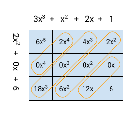
This pairing pattern becomes visually clear with a sliding diagram. Lay one polynomial out normally, and flip the other end-for-end so its constant term is first. Multiply aligned coefficients and sum them; this gives the product's constant term. Then slide the flipped polynomial one position, repeat, and you get the coefficient of x. Continuing this slide-and-multiply process yields each successive coefficient of the product.

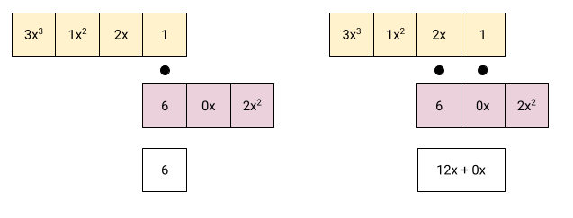
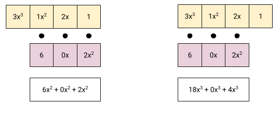
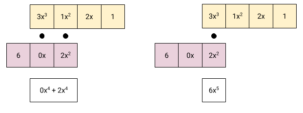
The need to reverse one of the inputs is a direct consequence of the index sum i + (k − i) = k in the coefficient formula. As the index in one polynomial grows, the paired index in the other must shrink so that their sum stays fixed for the output term being computed.

How Convolution Arises in Signals and Systems

This procedure of flipping and sliding is exactly the discrete convolution operation. The connection becomes clear when working with linear time-invariant (LTI) systems in signal processing.

Signals, Systems, and the Impulse Response

A discrete signal is a sequence of numbers x[n], indexed by integers n. A discrete system maps an input signal to an output signal. Two properties make a system especially tractable:

• Linearity: The response to a scaled sum of inputs is the same scaled sum of individual responses.
• Time-invariance: Shifting the input in time shifts the output by the same amount, without changing its shape.

For an LTI system, knowing its response to a single discrete impulse — called the impulse response h[n] — is sufficient to determine its output for any input. The reasoning relies on decomposing the input into a sum of scaled and time-shifted impulses. Because the system is linear, the response to the full signal is the sum of the responses to each individual impulse; because it is time-invariant, the response to a shifted impulse is simply the shifted impulse response.

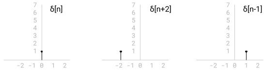
The signal x[n] can be written as the sum over k of x[k] · δ[n − k]. Using the system's linearity and time-invariance, the output y[n] becomes the convolution sum:

y[n] = Σ_k x[k] · h[n − k]

This is commonly written as y = x ∗ h.

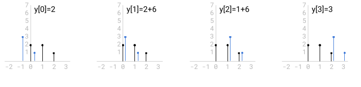
The index pairing in the convolution sum mirrors the polynomial case exactly. The index k in x increases, while the index n − k in h decreases. This is why one signal must be flipped relative to the other in the graphical sliding representation. Due to commutativity (which holds for convolution of sequences), either operand can serve as the flipped one.

A Worked Convolution Example

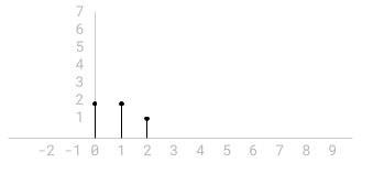
Take a finite input signal x = [2, 2, 1], and an impulse response h with nonzero values h[0] and h[1] only. Applying the convolution sum term by term:

• y[0] = x[0]·h[0]
• y[1] = x[0]·h[1] + x[1]·h[0]
• y[2] = x[1]·h[1] + x[2]·h[0]
• y[3] = x[2]·h[1]

All later output values are zero, since the input has no nonzero elements at indices beyond 2 and h has no nonzero elements beyond index 1.

Why Convolution Matters

The convolution operation shares many algebraic properties with ordinary multiplication, including commutativity, associativity, and distributivity over addition. Its most significant property, though, concerns the frequency domain. If F denotes the Fourier transform of a signal f, then the convolution theorem states:

F(x ∗ h) = F(x) · F(h)

Convolution in the time domain is equivalent to simple pointwise multiplication in the frequency domain. This fact underpins efficient convolution implementations that leverage FFT-based algorithms instead of direct summation. The theory runs deep, but the core insight is a unifying one: flipping, sliding, summing — whether over polynomial coefficients or impulse responses — all describe the same fundamental operation.