Querying the graph: breadth-first execution and async composition
Part 1 of this series covered the motivation for the Real-Time Distributed Graph (RDG) and the Apache Flink ingestion pipeline that turns streaming events into graph primitives; Part 2 covered the storage layer that handles billions of nodes and edges. This part covers the serving layer: how a constantly changing, billion-edge graph answers a wide variety of workloads in under 100ms.
Two query shapes, two pressures
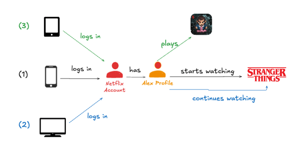
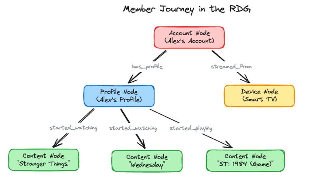
In the RDG's richer model, each account has multiple profiles. A member journey — Alex logging in on a smartphone to watch Stranger Things, continuing on a smart TV, then playing Stranger Things: 1984 on a tablet the next morning — produces a structure like this:
Queries vary along two independent axes: how wide they fan out per hop, and how deep they chain.
Shallow and wide
"Which devices has this account used to stream in the last 30 days?" starts at an Account node, traverses one streamed_from edge, and lands on Device nodes. A single hop, but a highly active account can fan out massively. The query layer must fetch hundreds of streamed_from edges, apply temporal filters on each edge's last_watch_timestamp property to keep only the last 30 days, and aggregate — all under 100ms.
Deep and narrow
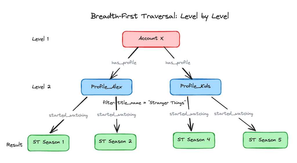
"For Account X, show me the Stranger Things viewing history across all profiles: which profiles watched it, what they watched, and when" walks Account → has_profile → Profiles → started_watching (filtered for title_name = "Stranger Things") → Content. The hard part is sequential dependency: the viewing history cannot be fetched until hop 1 has identified the profiles. If each hop costs 10ms of network time, that is 20ms of overhead before any data is processed. Hitting the sub-100ms goal required packaging multi-step logic into a single request. Real queries chain 3–4 hops across entity types, and the latency penalty of sequential execution grows with depth.
Shallow-wide queries stress I/O throughput; deep-narrow queries stress execution efficiency. The RDG serves tens of thousands of queries per second against a growing graph, so the design had to satisfy both.
Design decisions
Breadth-first over depth-first. Depth-first traversal traces one path to the end, backtracks, and tries another. In a distributed system where every hop is a network call, that misses batching opportunities: with five profiles, it would exhaust one profile's watched titles before touching the next. Breadth-first works one level at a time across all nodes — fetch all profiles, then started_watching edges for all profiles, then content details for all matching titles. Three rounds of parallel calls instead of sequential chains. The trade-off is memory: each level is held in memory at once, so cost scales with level width. Per-edge-type limits bound each hop, keeping even high fan-out frontiers manageable.
Async-first over thread-per-request. Latency is dominated by I/O — storage reads, enrichment calls, cache waits. A thread-per-request model pins a thread to each in-flight query, idle most of the time; thousands of concurrent queries would need thousands of mostly blocked threads. The pipeline is instead built on asynchronous composition: a small set of dedicated thread pools (16–24 threads total) handles thousands of concurrent requests because no thread ever blocks on I/O.
Selective caching. Account plan type and content metadata change on the order of hours or days; who watched what and when changes constantly. Stable data touched by many queries lives in a distributed cache (EVCache) with TTLs tuned to volatility. The team started by caching aggressively, tracked hit rates and stale-data incidents, and adjusted TTLs to how fast node types actually changed — reaching 70–80% hit rates on node lookups by caching only nodes that are frequently accessed and slow to change.
Opt-in, fail-open enrichments. Clients specify exactly which external data they want per request; a relationship check doesn't need title artwork. If an enrichment service is slow or unavailable, the graph data is returned without it.
Eventual consistency. Most queries ask what a member has done recently, not what happened in the last millisecond. Reading from the nearest replica avoids coordination overhead, though the RDG is not the source of truth for the data it holds.
Three layers
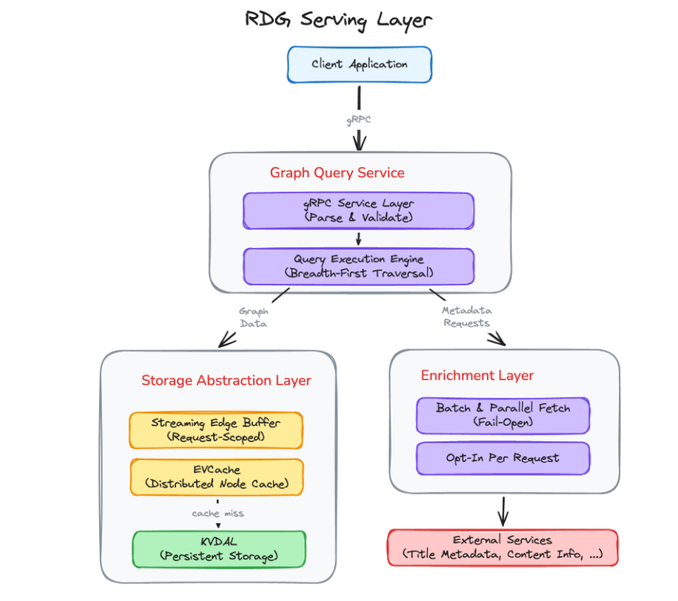
The Graph Query Service is the entry point: it accepts gRPC requests, validates the traversal specification, and hands it to the execution engine, which orchestrates breadth-first traversal — expanding one level at a time, applying filters and limits at each hop, and composing all I/O asynchronously. The Storage Abstraction Layer sits between the engine and KVDAL, providing node lookups and edge retrieval, handling streaming for large adjacency lists, and managing node caching in EVCache. The Enrichment Layer fetches external metadata on demand, batching requests, running them in parallel with graph data assembly, and degrading gracefully when a source is unavailable.
Requests flow through the layers in sequence: parse into an execution plan, walk the graph level by level, merge enrichments if requested, then serialize the response.
Following one query end to end
Take the deep-narrow example as a 2-hop traversal:
- Account X →
has_profile→ Profiles - Profiles →
started_watching→ Content (filtered for "Stranger Things")
Interpreting the request
Before touching storage, the engine merges a hierarchy of filters and limits — application-level defaults down to per-edge-type overrides — into a concrete plan specifying hop count, edges per hop, history window, and recency preference. Resolving this upfront prevents over-fetching downstream.
Reading from storage
Edges are organized as adjacency lists: for each node, a compact list of connections by edge type, so Account_X: has_profile → [Profile_Alex, Profile_Kids, …]. "Get all profiles for Account X" becomes a direct lookup into a small, well-indexed slice rather than a scan across billions of edges. In the example, the first hop returns just two profiles.
The second hop is the interesting one: each profile can have many started_watching edges, and loading a full adjacency list at once would spike latency and memory. Adjacency lists are treated as streams rather than blobs. The storage layer returns a profile's started_watching edges in batches of 100; filters are applied as each batch arrives, and reading stops once the query's limits (max_edge_cnt, lookback window) are satisfied. For Profile_Alex, roughly 500 edges — months of history — stream in; each batch is filtered for Stranger Things and anything older than 30 days, and after a few batches the handful of matching sessions has been found. Filtering happens at the source and no more data is materialized than needed.
Walking level by level
Level 1 pulls has_profile edges from Account X, yielding Profile_Alex and Profile_Kids as the frontier for Level 2 — one small lookup taking a few milliseconds. At Level 2, started_watching edges are fetched for each profile in parallel and filtered for Stranger Things as they stream, rather than exhausting one profile's full history before starting the next. The result: Profile_Alex watched seasons 1 and 2, Profile_Kids watched season 4 — a handful of sessions in roughly one storage round trip.
Parallelizing within each phase and regrouping gives predictable resource usage (a known number of requests per level), maximum parallelism (all frontier nodes processed together), and one round trip per level rather than per path. A 2-hop query becomes two rounds of parallel lookups instead of hundreds of sequential ones.
Parallelism with bounds
At production fan-out, hundreds of queries doing level-wide parallel work could overwhelm storage. The engine is structured like a professional kitchen: specialized stations with their own capacity, so a slammed station doesn't stall the others. Dedicated thread pools handle node fetches, adjacency-list reads, and enrichments separately; at Level 2, calls route to the adjacency-list pool, where 8 workers stream and filter each profile's edges in parallel. On top of per-pool limits, adaptive concurrency limiting tracks global capacity: the limit rises gradually while healthy (100 in-flight, then 101, 102) and backs off by a larger step on timeouts or errors (100 down to 70). Opted-in enrichments, such as maturity ratings, are fetched in parallel on their own pool and merged; a slow source never blocks the query.
Filtering
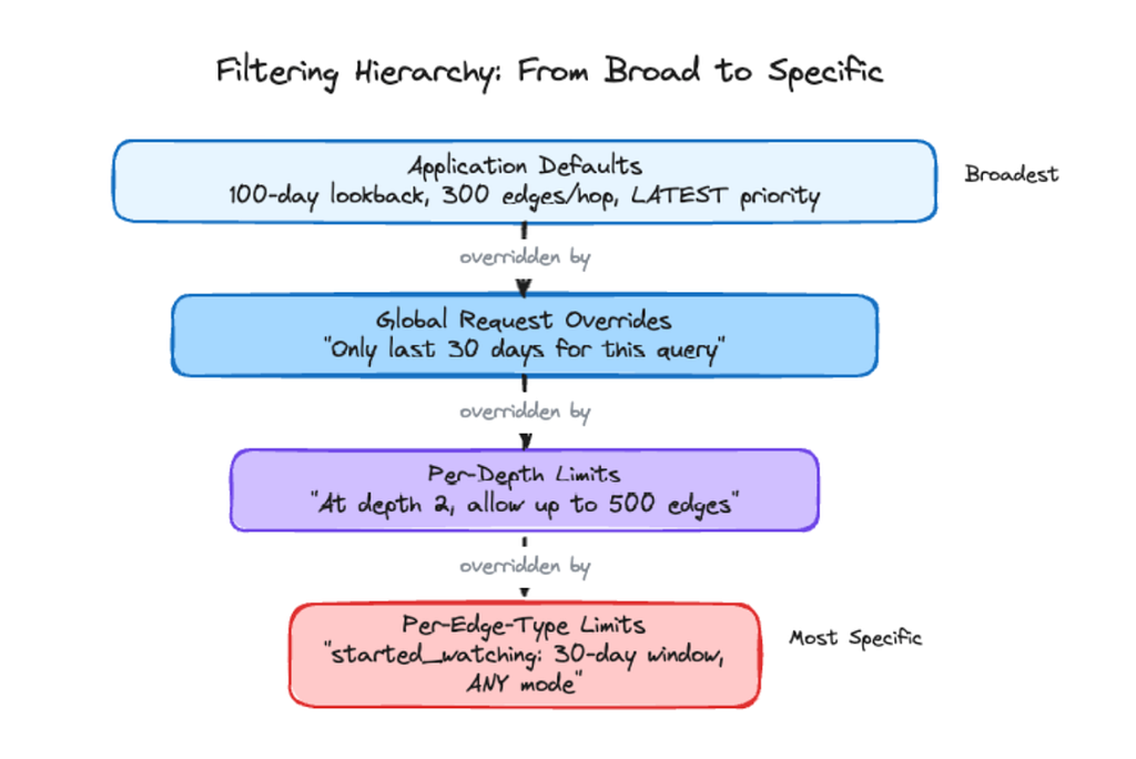
"Viewing history" means ignoring older activity, avoiding unnecessary edge fetches, and letting different teams define "recent enough." A layered override system starts from conservative defaults (100-day lookback, 300 edges per hop); requests override them globally, per-hop, or per-edge-type. Here the 100-day default applies broadly, but the caller sets 30 days for started_watching and the narrower rule wins. The same engine can apply a tight window to one edge type and full history to another in a single query.
When time filtering still leaves more edges than wanted — a profile rewatching an episode with pauses and resumes produces several — two selection modes decide what to keep. LATEST sorts edges by timestamp and keeps the newest up to the limit, for "what has this profile watched recently?" ANY takes whichever edges it encounters first, unsorted: faster, and sufficient for "has this profile ever watched Stranger Things?" Teams default to LATEST and switch specific edge types to ANY when any proof suffices.
For our query, the time filter narrows to 30 days, edge-count limits prevent response flooding, and LATEST picks the most recent session per title — yielding the profiles that watched Stranger Things in the last month, the seasons and episodes watched, and the most recent session for each.
Caching hot nodes
Account, Profile, and Content nodes rarely change, yet each storage call costs a network round trip; repeated lookups across thousands of queries per minute add infrastructure cost and tail latency. Hot nodes likely to reappear are held in a distributed cache, so "What is this node?" is answered from memory. On a cold first run of the Stranger Things query, everything is fetched and cached as it goes; a later query — "Show me everything Account X's profiles have watched in the last 7 days, and flag anything rated TV-MA on the kids profile" — finds many nodes already cached. Adjacency lists and edges still hit storage, but node lookups are lighter.
Not every node deserves a slot. The RDG prunes old activity after a retention window, so caching a node about to be deleted wastes memory. The policy weighs a node's last activity timestamp, the graph's retention period (e.g., 100 days), and the cache TTL (e.g., 30 days): a node last active 99 days ago expires from the graph in a day, so a 30-day TTL makes no sense and the node is skipped. Cache capacity stays with active nodes, and repeated traversals over the same part of the graph keep getting cheaper.
Measured behavior
The serving layer sits in front of 8 billion nodes and 150 billion edges. Single-hop queries return at a P50 of 15–30ms with P99 under 100ms; 3-hop traversals return at a P99 between 100–150ms. Breadth-first execution and per-level parallelism keep these numbers stable as fan-out grows, and because no thread ever blocks on I/O, thousands of concurrent requests flow through just 16–24 threads across the dedicated pools. When load spikes, the concurrency limiter lets work queue briefly, raising capacity slowly and backing off aggressively. Popular entities achieve 70–80% cache hit rates, which translates to roughly 3–4x fewer storage calls on common query paths.
What the team learned
Async composition changed the economics more than expected: it was intended to help latency, but a serving layer that would have needed hundreds of threads per instance now runs on 16–24. The trade-off is debuggability — async stack traces are hard to read and exceptions can get lost in future chains — which the team offset with per-stage metrics measured at validation, storage, enrichment, and end-to-end, so a slow stage is identifiable.
Caching took longer to get right. The first instinct, caching everything in EVCache and letting TTLs handle freshness, wastes memory on nodes about to expire from the graph anyway; the breakthrough was matching TTLs to volatility, with stable properties getting long TTLs and nodes near the end of their retention window not cached at all.
The filtering hierarchy came out of frustration: every new use case once meant a code change, with one team wanting a 7-day lookback, another 90 days, a third different limits at different depths. The layered override system — application defaults, global overrides, per-depth limits, per-edge-type limits — took real effort but eliminated a class of feature requests, and teams now tune their own queries without touching engine code.
Principles that generalize
- Think in frontiers, not features. Let callers describe the frontier to explore; let the system decide how to walk it efficiently.
- Filter early. Every byte fetched but unused is wasted I/O. Push filters and limits as close to storage as possible.
- Parallelize deliberately. Unbounded concurrency feels fast until it overwhelms dependencies. Set explicit limits, monitor them, and treat concurrency as a dial, not a switch.
- Cache as a first-class design choice. Decide what is worth remembering, for how long, in line with data volatility, and don't cache what is about to expire.